A New Empirical Relation between Surface Wave Magnitude and Rupture Length for Turkey Earthquakes

Many practical problems encountered in quantitative oriented disciplines entail finding the best approximate solution to an over determined system of linear equations. In this study, it is investigated the usage of different regression methods as a theoretical, practical and correct estimation tool in order to obtain the best empirical relationship between surface wave magnitude and rupture length for Turkey earthquakes. For this purpose, a detailed comparison is made among four different regression norms: (1) Least Squares, (2) Least Sum of Absolute Deviations, (3) Total Least Squares or Orthogonal and, (4) Robust Regressions. In order to assess the quality of the fit in a linear regression and to select the best empirical relationship for data sets, the correlation coefficient as a quite simple and very practicable tool is used.

A list of all earthquakes where the surface wave magnitude (Ms) and surface rupture length (L) are available is compiled. In order to estimate the empirical relationships between these parameters for Turkey earthquakes, log-linear fit is used and following equations are derived from different norms:

for L₂ Norm regression (R²=0.71),

for L₁ Norm regression (R²=0.92),

for Robust regression (R²=0.75),

for Orthogonal regression (R²=0.68),                           

Consequently, the empirical equation given by the Least Sum of Absolute Deviations regression as  with a strong correlation coefficient (R²=0.92) can be thought as more suitable and more reliable for Turkey earthquakes. Also, local differences in rupture length for a given magnitude can be interpreted in terms of local variation in geologic and seismic efficiencies.  Furthermore, this result suggests that seismic efficiency in a region is dependent on rupture length or magnitude. 

Resumen

Muchos problemas prácticos encontrados en las disciplinas de orientación cuantitativa implican encontrar la mejor solución aproximada para un sistema determinado de ecuaciones lineales. En este estudio se investiga el uso de diferentes métodos de regresión tanto teóricos como prácticos y la herramienta de estimación correcta con el fin de obtener la mejor relación empírica entre la magnitud de onda superficial y la ruptura de longitud para los terremotos en Turquía. Para este propósito se hace una comparación detallada a partir de cuatro normas diferentes de regresión: (1) mínimos cuadrados, (2) mínimas desviaciones absolutas, (3) mínimos cuadrados totales y (4) regresiones robustas. Con el fin de evaluar la regresión lineal adecuada y seleccionar la mejor relación empírica de grupos de datos empíricos, la correlación de coeficiente es una herramienta simple y muy práctica. Se compiló una lista de todos los terremotos donde se cuenta con la magnitud de onda superficial (Ms) y la ruptura de longitud superficial (L). Con el fin de determinar las relaciones empíricas entre estos parámetros para los terremotos de Turquía, se utiliza la regresión lineal adecuada y las siguientes ecuaciones se derivan de diferentes reglas.

Ms = 1.02* LogL + 5.18, para la regresión normal L₂ (R²=0.71),

Ms = 1.15* LogL + 4.98, para la regresión normal L₁ (R²=0.92),

Ms = 1.04* LogL + 5.15, para la regresión robusta (R²=0.75),

Ms = 1.25* LogL + 4.86, para la regresión ortogonal (R²=0.68).

Por consiguiente, la ecuación empírica dada por la regresión de desviaciones mínimas absolutas es con un fuerte coeficiente de correlación (R²=0.92) que sería más apropiado y más confiable para los terremotos de Turquía. También, las diferencias locales en la ruptura de longitud para una magnitud dada puede ser interpretada en términos de eficiencia sísmica y geológica en la variación local. Además, el resultado sugiere que la eficiencia sísmicaen una región depende de la ruptura de longitud o de la magnitud.

SEISMOLOGY

Serkan Öztürk¹,*

¹Gümüşhane University, Department of Geophysics, TR-29100, Gümüşhane, Turkey

*Corresponding author: Serkan ÖZTÜRK
Gümüşhane University, Department of Geophysics, TR-29100, Gümüşhane / Turkey. Email address: serkanozturk@gumushane.edu.tr - Phone: +90 456 233 74 25 / 26 - Fax: +90 456 233 10 75

Record
Manuscript received: 27/01/2014 Accepted for publication: 01/06/2014

---

ABSTRACT

Ms = 1.02* LogL + 5.18, for L₂ Norm regression (R²=0.71),

Ms = 1.15* LogL + 4.98, for L₁ Norm regression (R²=0.92),

Ms = 1.04* LogL + 5.15, for Robust regression (R²=0.75),

Ms = 1.25* LogL + 4.86, for Orthogonal regression (R²=0.68),

Consequently, the empirical equation given by the Least Sum of Absolute Deviations regression as Ms = 1.15* LogL + 4.98 with a strong correlation coefficient (R²=0.92) can be thought as more suitable and more reliable for Turkey earthquakes. Also, local differences in rupture length for a given magnitude can be interpreted in terms of local variation in geologic and seismic efficiencies. Furthermore, this result suggests that seismic efficiency in a region is dependent on rupture length or magnitude.

Key Words: Turkey, correlation coefficient, L₁, L₂, Orthogonal, Robust regression

Palabras clave: Turquía; coeficiente de correlación; L₁, L₂; regresión ortogonal; regresión robusta.

---

Introduction

The regression is one of the most used tools in establishing the relationship between a response and an explanatory variable in applied statistics. An effective and accurate curve fitting method plays an important role and serves as a basic module in many scientific and engineering fields. There exists vast literature about the regression problem in mathematics, statistics and computer science and there are many statistical regression methods for this purpose. Also, many software packages have allowed the practitioners to use the regression estimators to easily fit the data sets in order to determine whether or not there exists a relationship between hypothesized predictor or independent variables and some response or dependent variable (Giloni and Padberg, 2002).

There are a number of regression methods in the literature such as L₂ Norm or Least Squares Regression (Cadzow, 2002), L₁ Norm or Least Sum of Absolute Deviations Regression (Giloni and Padberg, 2002), Total Least Squares or Orthogonal Regression (Carroll and Ruppert, 1996), Robust Regression (Huber, 1964), Principle Components Regression (PCR, Maronna, 2005), Geometric Mean Regression (GMR, Leng et al. 2007), Least Trimmed Squares Regression (LTS, Rousseeuw and Leroy, 1987) and Covariate Adjusted Regression (CAR, Şentürk and Nguyen, 2006). The primary objective of this paper is to make an investigation on the usage of the best approximate regression solution to linear equations as a theoretical and practical estimation tool. For this purpose, a study on the comparison among the first four regression methods above is made in order to find the most suitable standard statistical model. The other methods such as PCR, GMR, LTS or CAR are not discussed since such kind of methods are described for more specific fields and they have not common use in geophysical investigations. Finally, these four different regression models are applied to Turkey earthquakes in order to determine more reliable and an up to date empirical relationship between surface wave magnitude and rupture length.

Brief description of the algorithms for regression techniques

There are different distance functions or metrics which can be utilized to perform a linear regression. Therefore, the original problem is categorized under the class of mathematical problems. In order to solve these problems, a remarkably wide range of mathematical techniques can be found in the literature. However, the aim of this study is not to discuss the mathematical details of the regression methods. Because the main goal of this work is to test different regression methods and to find the most suitable empirical relationship between surface wave magnitude and rupture length for Turkey earthquakes, a brief and general reviews of four different regression approaches are given in this section as well as their fundamental statistical properties and qualities of fits.

The linear regression problem is certainly one of the most important data analysis situations. In order to formulate a linear regression model, it is assumed that there are n measurements on the dependent variable y and some number p≥1 of independent variables χ₁,……., χ_p of each one for which it is known n values as well. It is defined by Giloni et al., (2006) as follows:

where y Є R is a vector of n observations and X is an n x p matrix of real frequently referred to as the design matrix. Furthermore, x₁,…….,x_p are column vectors with n components and x¹,…….,xⁿ are row vectors with p components corresponding to the columns and rows of X, respectively. The statistical (or hypothesized) linear regression model is given:

where ß^T = (ß₁,........,ß₂) is the vector of parameters of the linear model and ε^T = (ε₁,........,ε₂) a vector of n random variables corresponding to the error terms in the asserted relationship. An upper index T denotes "transposition" of a vector or matrix. In the statistical model, the dependent variable y, thus, is a random variable for which we obtain measurements that contain some "noise" or measurement errors that are captured in the error terms e. On the other hand, for the numerical problem that we are facing, it can be written:

where given some arbitrarily fixed parameter vector β, the components r_i of the vector r^T = (r₁,........,r₂) are the residuals that result, given the observations y, a fixed design matrix X, and the chosen vector ß Є R^p . The residuals r are thus in terms of the statistical model, realizations of the random error terms e given the particular observations y and parameter settings β. Given y and X, the general objective in linear regression is to find parameter settings ß Є R^p such that some appropriate measure of the dispersion of the resulting residuals r Є Rⁿ is as small as possible (Giloni and Padberg, 2002).

L₂ Norm or Least Squares Regression

Least squares regression (L₂ norm) is the most well-known and the most basic form of the least squares optimization problems. So, it has found many applications in mathematics and statistical data analyses as well as the other scientific fields. This statistical linear regression model has been studied intensively for well over 200 years now and under the assumption of a normal (or Gaussian or exponential) distribution of the error terms e an impressive statistical apparatus has been created to assess the goodness of fit, the quality of individual and/or subsets of the regression coefficients, as well as other statistical properties of the linear regression model. If and when the error terms in the linear regression model do indeed follow a normal distribution, then the least squares regression estimates are "the best estimators" under most acceptable criteria. Thus, this approach is particularly helpful in all those situations involving the study of large data sets, handling large samples with a consistent numbers of outliers (e.g., Cadzow, 2002; Giloni and Padberg, 2002).

L₁ Norm or Least Sum of Absolute Deviations Regression

The least squares linear regression estimator is well-known to be highly sensitive to outliers in the data and as a result many more robust estimators have been proposed as alternatives. One of the earliest proposals was the least-sum of absolute deviations (L₁) regression, where the regression coefficients are estimated through minimization of the sum of the absolute values of the residuals. L₁ regression is called in the literature by a multitude of names that all mean the same: LAD (least absolute deviation), LAE (least absolute error), LAV (least absolute value), LAR (least absolute residual), LSAD (least sum of absolute deviations), MAD (minimum absolute deviation), MSAE (minimum sum of absolute errors), and so forth.

An important advantage of L₁ regression over L₂ regression is its robustness. For the unconstrained problem it is well known that the L₁ regression estimator can resist a few large errors in the data y (Shi and Lukas, 2005). The use of L₁ norm criterion is appropriate when it is suspected that a small portion of the data being analyzed is unreliable (i.e., contains data outliers). The L₁ norm criterion has the capability of effectively ignoring a few bad data points while emphasizing the majority of data points which more properly reflect the true nature of the data (Cadzow, 2002). One can see Huber (1987) for further discussion of the L₁ approach in robust estimation.

Total Least Squares or Orthogonal Regression

One of the most widely known techniques for errors-in-variables estimation in the simple linear regression model is orthogonal regression, also sometimes called as the functional maximum likelihood estimator under the constraint of known error variance ratio. In ordinary linear regression, the goal is to minimize the sum of the squared vertical distances between the y data values and the corresponding y values on the fitted line. In orthogonal regression the goal is to minimize the orthogonal (perpendicular) distances from the data points to the fitted line.

This well-known orthogonal regression estimator is an old method and derived in many studies such as Weisberg (1985), Carroll and Ruppert (1996) and Leng et al., (2007). The use of orthogonal regression must include a careful assessment of equation error, and not merely the usual estimation of the ratio of measurement error variance. Thus, when its assumptions hold, the orthogonal regression is a perfectly justifiable method of estimation. However it often lends itself to misuse by the unwary as a method, because orthogonal regression does not take equation error into account.

Robust Regression

The most serious problem with least squares regression is non-robustness to outliers. In particular, if you have one extremely bad data point, it will have a strong influence on the solution because outliers can have a large influence on the regression parameters. A simple remedy is to iteratively discard the worst-fitting data point, and re-compute the least squares fit to the remaining data. Another approach, termed robust regression, is to employ a fitting criterion that is not as vulnerable as least squares to unusual data. The most common general method of robust regression is M-estimation, introduced by Huber (1964).

Nonlinear regression models play an important role in many fields. For estimating the parameters of a nonlinear model, the classical least squares method is commonly used in many cases. However, it is well known that these classical methods are often very sensitive to outliers and other departures from the underlying distribution. Most robust developments on the estimation of regression models are based on the generalizations of least squares or maximum likelihood methods. Robust regression procedure is less influenced by extreme values. In assessing the behavior of robust regression estimates, however, the techniques of small sample asymptotes can be very useful. The literature on the robust regression dates back to Huber (1964). Some of the robust techniques are also discussed in many studies such as Huber (1981), Sinha et al., (2003) and Abdelkader et al., (2010).

Determination of Correlation Coefficient for Regressions

One of the most important problems in regression analyses is the selection of an appropriate probability distribution for a given data set, which can give reasonably accurate and robust estimates. As shown in the literature, there is no certain rule for selecting the appropriate distribution or parameter estimation techniques for a given data set and various distributions should be applied and the best-fitting model should be selected. Thus, choosing the best-fitting model is quite an important procedure in frequency analysis. In most cases, the selection of an appropriate distribution is based on goodness-of-fit assessment. The goodness-of-fit technique can be described as the method for examining how well sample data agree with an assumed probability distribution as its population. Several goodness-of-fit tests are developed and used in engineering decision-making. Selection criteria among those methods, the determination of correlation coefficient (R² or sometimes r is used) has been known as a powerful and conceptually simple method. Although the R² is solely based on the covariance penalty, it plays an important role in model fit assessment. It should certainly not be used as a unique model fit assessor, but can provide a reasonable and rapid model fit indication (Heo et al. 2008).

More traditionally, for the linear regression model, a very simple fit indicator is, however, given by the determination of correlation coefficient R². If x is considered as random, it can be defined as the parameter that is the squared correlation between y and the best linear combination of the x. The R² is usually presented as the quantity that estimates the percentage of variance of the response variable explained by linear relationship with the explanatory variables. It is computed by means of the ratio:

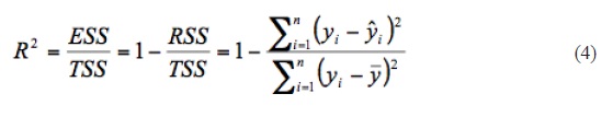
where ESS, TSS and RSS are the explained, total and residual sum of squares, respectively. When there is an intercept term in the linear model, this determination of correlation coefficient is actually equal to the square of the correlation coefficient between y_i and ŷ_i:

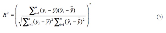
where y and ŷ denote the mean values of the observations y_i and the fitted quantiles ŷ_i, respectively. Equation (5) has a nice interpretation in that R² measures the goodness of fit of the regression model by its ability to predict the response variable, ability measured by the correlation. The correlation coefficient is location and scale invariant, and statistically independent of the mean, y, and standard deviation. Essentially, R² measures the linearity of the probability plot, providing a quantitative assessment of fit and it is assumed that the observations could have been drawn from the fitted distribution if the value of R² is close to 1.0 (Heo et al., 2008).

Some Characteristics of Earthquakes used in the Analysis and Main Geological Environments around these Earthquakes

Main goal of this study is to derive a relationship between the surface wave magnitude and rupture length for great earthquakes occurred in and around Turkey. For this purpose, the earthquakes whose surface wave magnitude are greater than 5.5 and occurred between 1905 and 2005 were used. Magnitude ranges vary from 5.5 to 8.0 and rupture length changes between 3 and 350 km for 63 earthquakes. These events and their detailed information can be found from different studies in the literature (e.g., Ambreseys and Jackson, 1998; Nalbant et al. 1998; Dewey, 1976). The epicenters of all earthquakes used in the analysis and whole tectonics are plotted in Figure 1. In addition, some principle characteristics of several earthquakes and geological environments around these earthquakes are briefly discussed in this section. Details of geological structure for whole epicenter regions are provided from the General Directorate of Mineral Research & Exploration (MTA, http://www.mta.gov.tr/v2.0/daire-baskanliklari/jed/index.php?id=500bas).

The 1912 Marmara (Mürefte Şarköy) earthquake was located between the Gulf of Saros and the Sea of Marmara. This earthquake was followed by several large aftershocks (August 10, 1912, Ms = 6.3; September 13, 1912, Ms = 6.9; September 27, 1912, Ms = 6.6) to the west of the main shock. The surface rupture pattern of this earthquake was reported as a complex with a substantial right-lateral strike-slip component. Nalbant et al., (1998) defined three fault segments with a vertical dip: the eastern one and middle ones have a reverse component, while the western one, bounding the Gulf of Saros, is pure strike slip. Geological formation around the related earthquakes is mainly composed of clastic and carbonate rocks. Another earthquake which is occurred in the same zone is the 1935 Marmara earthquake. This earthquake occurred on the southwest extremity of the Sea of Marmara, north of the Marmara Islands. Nalbant et al., (1998) modeled this earthquake as east-west striking normal faulting dipping to north. They adopted a dip of 45° and mean displacement of 0.85 m. Geological structure around this earthquake epicenter includes granitoid, schist, phillite, marble, metabasic rocks etc.

There are two earthquakes in Burdur region. The first one occurred in 1914 and the other one in 1971. These two earthquakes were located approximately in the same coordinates. The first earthquake occurred on the northeast segment of Burdur Fault and the other occurred on the southwest of Burdur Lake. Focal mechanisms of the 1914 and 1971 Burdur earthquakes are very similar. Fault plane solution of the 1914 earthquake indicates normal faulting with a dip of 35° and a mean displacement of 1.6 m. Focal mechanism of the 1971 earthquake shows pure normal faulting with a dip of 35° and a displacement of 0.7 m (Taymaz et al. 1991). Main geological structure around these epicenters includes undifferentiated quaternary, continental clastic rocks and undifferentiated continental clastic rocks.

The 1919 Soma (Manisa) earthquake, in the south of the North Anatolian Fault, occurred in the eastern part of the Bakırçay normal fault zone which also ruptured during the 1939 Bergama earthquake. As east-west normal faulting and right-lateral strike-slip faulting are found in the area, Nalbant et al., (1998) modeled this earthquake as right lateral normal fault dipping to north. They assumed a dip of 45° and mean displacement of 1.4 m for this earthquake. Geological structure around this earthquake epicenter is given as undifferentiated quaternary by MTA. The second earthquake in the same region is the 1969 Demirci (Manisa) earthquake. It was located on the North Anatolian Fault at the easternmost part of the Sea of Marmara, Mudurnu Valley. Its fault plane solution based on teleseismic body-waveform inversion shows a E-W dextral strike-slip faluting mechanism (Taymaz et al. 1991). Nalbant et al., (1998) modeled this earthquake with dipping south at 45° and a displacement of 0.35 m. Geological formation around this epicenter includes continental clastic rocks, dacite, rhyolite, rhyodacite, migmatite and gneiss. The other earthquake in the same region is March 28, 1969, Alaşehir earthquake. This event occurred in the Gediz River Valley with 30 km surface rupture and extending from NW through Alaşehir to SE. The fault plane solution of this earthquake shows a normal faulting with a dip of 32° and a mean displacement of 0.61 m (Eyidogan and Jackson, 1985). Geological structure around this epicenter includes undifferentiated quaternary, alluvial fan, slope debris, etc.

The 1924 Altıntaş (Kütahya) earthquake occurred in the western Anatolia, east of the 1970 Gediz (Kütahya) earthquake. The east-west normal faulting is a dominant mechanism in this region and was associated with 1956 Eskişehir and the 1970 Gediz earthquakes. Nalbant et al., (1998) assumed that this event occurred on an east-west, normal fault located near epicenter with a dip of 45° which is compatible with the known tectonics of the area and mean displacement of 0.2 m. Geological environments near the epicenter of this earthquake consist of undifferentiated quaternary, gneiss, metagranite, schist, marble, amphibolite etc. Another earthquake around this area is 1928 Emet earthquake and they show a similar tectonic environment. In this region, NNW-SSE striking normal faults dipping to the ENE were reactivated during the earthquakes in 1970 and 1944 (Nalbant et al. 1998). Different from 1924 Altıntaş earthquake region, geological structure includes continental carbonate rocks. The third earthquake in the same region is 1944 Şaphane earthquake. This earthquake was located in the western Anatolia, southwest of Gediz and also ruptured during the 1970 Gediz earthquake. (Nalbant et al., 1998) modeled this earthquake as NNW-SSE normal fault with a dip of 45° and a mean displacement of 0.2 m. Geological formation around this epicenter is formed by continental clastic rocks and pyrolastic rocks. The fourth earthquake in this region is 1970 Gediz earthquake which is occurred in the western Anatolia, east of the Simav fault system. Ambraseys and Tchalenko (1972) mapped about 45 km of complicated normal faulting trending both to the NNW-SSE and east-west down thrown to the east and north. Eyidogan and Jackson (1985) modeled the seismograms of this earthquake using three main subevents. The first subevent occurred on 15 km long NNW-SSE segment with a mean displacement of 1.6 m and a dip of 35°. It then triggers the second subevent which ruptures the 24 km long east-west segment with a mean displacement of 2.4 m and a dip of 35°. All the remaining complexity of seismograms can be explain by slip on a~15° dipping fault extending the second fault segment from a depth of 12.5 to 17.5 km. Geological structure around this epicenter includes continental clastic rocks.

The 1930 Hakkari earthquake was located near the Iran-Turkey border. Focal mechanism of this earthquake display a right-lateral strike-slip faulting with a normal fault component with a dip of 36° and a mean displacement of 4.5 m (Ambraseys and Jackson, 1998). Geological formation around this epicenter includes pyroclastic rocks, basalt, ophiolitic melange.

The Bergama (İzmir) earthquake was located in 1939 near the coast in the western Anatolia, at the western extremity of the Bakırçay normal fault zone. The focal mechanism solution indicates east-west normal faulting (Ritsema, 1974). Nalbant et al., (1998) modeled the rupture of this event to the dip at 45° and a mean displacement of 0.75 m. Geological formation around this epicenter consists of generally undifferentiated quaternary and undifferentiated volcanic rocks (generally andesitic). The other earthquake in the same region is the 2005 Urla earthquake. This earthquake occurred in the Gulf of Sığacık, in a region dominated by N–S extension and bounded by well-documented graben structures. The focal mechanisms of the 17 October 2005 earthquake seismic sequence show pure strike-slip motions in the Gulf of Sığacık and normal faulting combined with considerable strike-slip motion in the north and in the south (Benenatos et al. 2006). Geological structure around this epicenter includes neritic and lacustrine limestone, marl, shale etc.

The 1939 Erzincan Earthquake occurred on the North Anatolian Fault Zone was one of the most active strike-slip faults in the world. This earthquake nucleated on the eastern portion of the rupture. Main body of the rupture extended along the master strand of the NAF between Erzincan and Niksar basins. However, a part of 76 km-long the westernmost portion of the rupture directed towards on the Ezinepazarı fault. Ambraseys and Zapotek (1969) stated that fault plane for this earthquake shows as a right-lateral mechanism. Burumbaugh and Pınar (2001) stated that the first-motion fault plane solution obtained at the epicentral location was a fault plane parallel to the easternmost surface rupture segment with a dip of 80° and mean displacement of 3.7 m. The other large earthquake in this region is the 1992 Erzincan earthquake. This earthquake is located within a key region of eastern Anatolia, which displays both expulsion of the Anatolian block towards the west and regional N-S convergence due to the Arabian-Eurasian collision. The main focal mechanism is strike-slip with a slight normal component a dip of 68° and mean displacement of 1.0 m. (Fuenzalida et al. 1997). Main geological environments around these epicenters consist of undifferentiated quaternary, peridotite, slope debris, cone of dejection etc.

The 1942 Bigadiç (Balıkesir) earthquake was located in the western Anatolia, south of Balıkesir. In this region, normal faults strike east-west and dip toward the north (Westeway, 1990). Nalbant et al., (1998) modeled the rupture of this earthquake as a12.5 km long normal fault and assume a dip of 45° and a mean displacement of 0.35 m. Geological structure around this earthquake epicenter includes undifferentiated quaternary, undifferentiated volcanic rocks, dacite, rhyolite, rhyodacite. Another event in the same city is the 1944 Ayvacık earthquake. This earthquake occurred near the Edremit Gulf. The southern branch of the North Anatolian Fault reaches the Aegean Sea through the Edremit Gulf. The poorly constrained focal mechanism indicates nearly pure strike-slip (Ritsema, 1974). However, Nalbant et al., (1998) stated that it could have a normal component with an oblique slip on a 60° south dipping fault and a mean displacement of 1.6 m. Geological formation around this epicenter consists of continental clastic rocks.

The 1942 Niksar-Erbaa (Tokat) earthquake was located in the Erbaa-Niksar area, in the North Anatolian Fault Zone from Niksar in the Kelkit River Valley to the Yeşilırmak River west of Erbaa. Focal mechanism of this earthquake shows right-lateral strike-slip faulting with a dip of 90° and a mean displacement of 1.8 m (Ambraseys and Jackson, 1998). Geological structure around this epicenter includes undifferentiated quaternary, undifferentiated continental clastic rocks, schist, phyllite, marble and metabasic rocks.

The 1943 Hendek (Adapazarı) earthquake occurred in the east of the Sea of Marmara in the Mudurnu valley, 15 km north of the 1967 rupture. The focal mechanism of this earthquake is almost pure strike-slip motion parallel to the North Anatolian Fault. Nalbant et al., (1998) modeled this event as a 16 km long right-lateral faulting with a dip of 90° and with 0.75 m of displacement (Ambraseys and Jackson, 1998). Geological structure around this earthquake epicenter consists of undifferentiated volcanic rocks, clastic and carbonates rocks.

The 1943 Tosya-Ladik (Samsun) earthquake occurred near Tosya, Kastamonu province, in northern Turkey. Surface faulting was observed in section of the North Anatolian Fault Zone from the Destek Gorge west of Erbaa to the Filyos River. Focal mechanism of this earthquake shows right-lateral strike-slip faulting with a dip of 80° and with a mean displacement of 2.0 m (Wells and Coppersmith, 1994). Geological structure around this earthquake epicenter is formed by undifferentiated quaternary.

The 1944 Gerede (Bolu) earthquake was located on the North Anatolian Fault. Nalbant et al., (1998) modeled this earthquake with a right-lateral strike-slip fault and with slip distribution 3.5 m to the west and decreases to 1.5 m in the east. Geological formation around this epicenter consists of clastic and carbonate rocks. Another event in the same region is 1957 Abant earthquake. This earthquake occurred on the North Anatolian Fault. The focal mechanism of this earthquake indicates strike-slip faulting (McKenzie, 1972). Nalbant et al., (1998) modeled this event with an average of 2.5 m strike-slip motion. Geological structure near this earthquake epicenter is formed by clastic and carbonate rocks, alluvial fan, slope debris, cone of dejection etc. The other event in near region is July 22, 1967, Mudurnu earthquake. This earthquake occurred in the east of the Sea Marmara on the North Anatolian Fault. The focal mechanism is given as a pure, east-west, strike slip faulting and mean displacement of 2.5 m (Nalbant et al. 1998). Geological environments near this epicenter include undifferentiated quaternary, undifferentiated volcanic rocks, clastic and carbonate rocks.

The 1946 Varto-Hınıs (Muş) earthquake occurred in Varto district, province of Muş. Focal mechanism of this earthquake shows right-lateral strike-slip faulting with a dip of 58° and a mean displacement of 0.3 m (Ambraseys and Jackson, 1998). The other earthquake in the same region, the Varto-Üstükran earthquake of August 19, 1966, was located near the east end of the North Anatolian Fault System in Turkey, very near where an earlier, less intense earthquake had caused damage in May 31, 1946. Fault plane solution displays right-lateral strike slip faulting that having an extension of normal fault component with a dip of 65° and a mean displacement of 0.3 m (Ambraseys and Jackson, 1998). Geological formation around these epicenters includes continental clastic rocks, pyroclastic rocks, basalt, slope debris, cone of dejection etc.

The 1951 Kurşunlu (Çankırı) earthquake was related with North Anatolian Fault and occurred in the eastern tails of the İsmetpaşa segment. Focal mechanism of this earthquake shows right-lateral strike-slip faulting with a dip of 60° and a mean displacement of 0.6 m (Nalbant et al. 1998). The June 6, 2000 Orta (Çankırı) earthquake was located about 25 km south of the North Anatolian Fault Zone. The epicenter of this earthquake is close to a restraining bend in the E-W striking right-lateral strike-slip fault that moved in the much larger earthquake of August 13, 1951 Kurşunlu earthquake. Fault plane solution of 2000 earthquake shows normal faulting with a left lateral component with a dip of 69° and a mean displacement of 0.82 m (Irmak, 2000). Geological structure around these epicenters includes undifferentiated volcanic rocks, basalt, lacustrine limestone, marl, shale etc.

The 1953 Yenice-Gönen earthquake was located between the Sea of Marmara to the north and the Edremit Gulf to the south. This earthquake ruptured the southern branch of the North Anatolian Fault. Focal mechanism of this earthquake indicates pure southwest-northeast right-lateral strike-slip faulting (Ambraseys, 1978). Nalbant et al., (1998) modeled this earthquake using the slip reaching 3.5 m in the eastern and dropping to both ends. Geological structure around this epicenter is formed by undifferentiated volcanic rocks, neritic limestone, schist and clastic rocks.

The 1956 Eskişehir earthquake was located in the western Anatolia, 30 km west of Eskişehir and 100 km north of Gediz. This earthquake occurred on the Eskişehir normal fault system (McKenzie, 1972). Fault plane solution indicates east-west normal faulting. Nalbant et al., (1998) modeled this event as resulting from the rupture of an east-west normal fault dipping to the north with an angle of 45° and a displacement of 0.30 m. Geological formation around this epicenter consist of undifferentiated ophiolitic rocks, schist, fillite, marble and metabasite.

The 1963 Yalova-Çınarcık earthquake was located in the southeast Sea of Marmara, north of the Yalova. The fault plane solution is given as pure northwest-southeast normal faulting (Taymaz et al. 1991). Nalbant et al., (1998) modeled this event as a normal fault dipping northward with a dip of 60° and displacement of 0.60 m. Geological structure around this earthquake epicenter includes continental clastic rocks, carbonate and clastic rocks.

The 1964 Manyas earthquake was located on the south of the Sea of Marmara between the Manyas Lake and the Ulubat Lake on the southern branch of the North Anatolian Fault. The focal mechanism solution shows east-west normal faulting (Taymaz et al. 1991). Nalbant et al., (1998) modeled this earthquake with a dip of 45° and a mean displacement of 1.2 m. geological environments around this epicenter includes undifferentiated quaternary and continental clastic rocks.

The first Aegean earthquake which occurred in 1965 was located in the Aegean Sea at the southwest extremity of the North Aegean Through. The focal mechanism indicates right lateral strike-slip faulting on a northeast-southwest plane (Taymaz et al. 1991). Nalbant et al., (1998) modeled this event with a slip of 0.6 m. The second earthquake in the same region is the 1967 Aegean earthquake which was located in the Aegean Sea at the northwest extremity of the Skyros Basin, south of the North Aegean Through. The predominantly normal faulting focal mechanism (Taymaz et al. 1991) defines two possible fault planes: one striking east-west with a dip toward the south, the other northwest-southeast with a dip toward the northeast. The major normal faults in the area bounding the western edge of Skyros Basin are oriented like the second nodal plane. Nalbant et al., (1998) modeled this earthquake as a northwest-southeast normal fault with a dip of 45° and a displacement of 0.70 m. The third earthquake is December 19, 1981, Aegean earthquake which occurred in the Aegean Sea, on the southern edge of the Skyros Basin. The fault plane solution shows right-lateral strike-slip faulting striking northeast-southwest (Taymaz et al. 1991). Nalbant et al., (1998) modeled this event with a dip of 79° and a mean displacement of 3.2 m. The fourth Aegean earthquake occurred in the southwest extremity of the Skyros basin on December, 27, 1981. Its focal mechanism also indicates right-lateral faulting striking northeast-southwest (Taymaz et al. 1991). Nalbant et al., (1998) modeled this event with a dip of 79° and a mean displacement of 0.75 m. The fifth earthquake which was located in the same region is January, 18, 1982, Aegean earthquake. This earthquake was located in the Aegean Sea, in the central part of the North Aegean Through. Its fault plane solution shows right-lateral strike-slip faulting on a northeast-southwest plane (Taymaz et al. 1991). Nalbant et al., (1998) modeled this event with a dip of 62° and a mean displacement of 2.25 m. The last event in this region is 1983 Aegean earthquake. This earthquake was located in Aegean Sea, just east of the previous one. The northeast elongation of the aftershock zone and the strike-slip focal mechanism are similar to the 1982 earthquake (Taymaz et al. 1991). Nalbant et al., (1998) modeled this event as a northeast-southwest right-lateral fault on the southern edge of the North Aegean Trough with dip of 83° and a displacement of 2.25 m. There is no information about the geological formation around these epicenters because these events occurred in the sea.

The 1967 Tunceli earthquake occurred in the part which is between Pülümür and Kalıova of North Anatolian Fault. Fault plane solution of this earthquake shows right-lateral strike-slip faulting with a dip of 88° and a mean displacement of 0.2 m (Ambraseys and Jackson, 1998). The 2003 Pülümür (Tunceli) earthquake occurred on the Pülümür fault that has 45° with the eastern part of the North Anatolian Fault. The epicenter of the earthquake was located at about 4.5 km W-SW Sağlamtaş village. Focal mechanism of this earthquake shows predominantly left-lateral strike-slip faulting that displayed a normal fault component with a dip of 71° and a mean displacement of 0.36 m (Ozener et al. 2010). Geological structure around these epicenters includes clastic and carbonate rocks, continental clastic rocks and undifferentiated volcanic rocks.

The Bartın (Zonguldak) earthquake of September 3, 1968 is the strongest instrumentally recorded earthquake to occur along the Black Sea margin in northwestern Turkey. The epicenter of the main shock was located 10 km north of Amasra, in the Black Sea. The fault plane solution of this earthquake shows a thrust faulting with a dip of 38° and a mean displacement of 0.2 m (Alptekin et al. 1986). Geological formation around this epicenter consists of continental clastic rocks, clastic and carbonates rocks, neritic limestone.

The May 22, 1971, Bingöl earthquake was centered near Bingöl. This earthquake produced surface breaks mostly along the southwestern half of the northeastern segment of the East Anatolian Fault between the Karlıova triple junctions. Earthquake mechanism of this event reveals left-lateral strike slip geometry with a dip of 45° and a mean displacement of 0.70 m (Taymaz et al. 1991). The second earthquake in the same region is May 01, 2003, Bingöl earthquake. This earthquake was located approximately 60 km southwest of the triple junction near Karlıova, where North Anatolian Fault and East Anatolian Fault intersect. Fault plane solution of this earthquake shows right-lateral strike-slip fault with a dip of 88° and a mean displacement of 0.9 m (Milkereit et al. 2004). Geological environments around these epicenters consist of undifferentiated volcanic rocks, schist, quvarzite, marble, phillite, etc.

The earthquake of March 27, 1975, Saros (Çanakkale) earthquake was located on the west of the Sea of Marmara in the Gulf of Saros, a pull-apart basin associated with the northern part of the North Anatolian Fault. Fault plane solution shows a strike-slip, normal fault (a dip of 55°), rupture with the right lateral plane ENE-WSW (Taymaz et al. 1991). Nalbant et al., (1998) modeled this earthquake as an oblique fault with a length of 20 km and displacement of 0.95 m. There is no information about the geological structure around this epicenter because this event occurred in the sea.

The Lice (Diyarbakır) earthquake of 1975 was located near the town of Lice, in the western part of the Bitlis Thrust Zone. The slip vector in this event is thus directed NE, and may be related to the Arabia-Turkey motion, rather than the Arabia-Eurasia motion (Moazami-Goudarzi and Akasheh, 1977). The mechanism of faulting for the Lice earthquake of September 6, 1975 is thrust fault with a dip of 50° and a mean displacement of 0.5 m (Wells and Coppersmith, 1994). Geological structure around this epicenter includes clastic and carbonate rocks.

The 1976 Çaldıran (Van) earthquake occurred about 100 km east of the junction between the North and East Anatolian Faults, extending from 3 km west of Sarıkök in the west to just west of Baydoğan in the east. Focal mechanism of this earthquake shows right-lateral strike-slip faulting with very small thrust component with a dip of 78° and a mean displacement of 2.05 m (Wells and Coppersmith, 1994). Geological formation around this epicenter includes undifferentiated quaternary, undifferentiated continental clastic rocks, alluvial fans, slope debris, moraine etc.

The 1983 Horosan-Narman (Erzurum) earthquake took place on the NE-SW trending Horosan Fault, between Horosan and Şenkaya about 60 km east of Erzurum basin. Its fault plane solution indicates left-lateral strike slip geometry with a small thrust component, with a dip of 64° and a mean displacement of 1.2 m (Wells and Coppersmith, 1994). Geological structure around this earthquake epicenter consists of pyroclastic rocks, undifferentiated volcanic rocks, and undifferentiated basic and ultrabasic rocks.

The Kars earthquake of 1988 December 7 was located within the Lesser Caucasus, which is dominated by a north-south compressive tectonics resulting from the young continental collision between the Arabian plate and Russian Platform. Focal mechanism of this earthquake was obtained as right-lateral strike-slip fault with a dip of 29° and a mean displacement of 1.6 m (Wells and Coppersmith, 1994). Geological formation around this epicenter includes undifferentiated continental clastic rocks.

The 1995 Dinar (Afyon) earthquake took place in the West Anatolian province, in the lakes region horst-graben system. Its epicenter is located near the Dinar-Çivril Fault. Focal mechanism of this earthquake indicates a normal faulting with a small lateral component with a dip of 56° and an average displacement of 0.2–0.4 m (Pınar, 1998). Geological structure around this epicenter consists of undifferentiated quaternary and neritic limestone. The other earthquakes in the same region occurred in the southwestern Turkey on December 15, 2000 (Sultandağı) and February 3, 2002 (Eber) earthquakes. This earthquake sequence took place on the Sultandağ Fault. The 2000 earthquake occurred on the Sultandağı Fault, near the city of Afyon in southwestern Turkey whereas the 2002 earthquake occurred on the northwestern segment of the Sultandağı Fault. Focal mechanisms of the 2000 earthquake indicate normal faulting with a slight left-lateral component with a dip of 41° and a mean displacement of 0.25 m. Focal mechanism of the 2002 earthquake shows normal faulting with a dip of 38° and a variable displacement between 0.6 and 1.0 m (Aksarı et al. 2010). Geological environments around these epicenters include undifferentiated quaternary, undifferentiated continental clastic rocks, marble and recrystallized limestone.

The 1998 Adana-Ceyhan earthquake occurred in southern Turkey with its epicenter close to the city of Adana, characterized by the advance of the Arabic plate towards the north and the consequent wedging of the Eurasian plate. This earthquake resulted by a left-lateral strike-slip faulting along the NE-trending East Anatolian fault system and other fault zones, parallel to it, in the west. Parameters of earthquake fault were given as 80° for dip and 0.37 m for mean displacement (Lekkas and Vassilakis, 1999; Aktar et al. 2000). Geological structure around this epicenter consists of undifferentiated quaternary.

The 1999 İzmit earthquake, one of the most destructive earthquakes in Turkey, was located in the western part of the North Anatolian Fault, in northwestern Turkey in the Gulf of İzmit region. The İzmit main shock occurred as a right-lateral strike slip faulting on an EW trending with a dip of 83° and a mean displacement of 5.0 m (Tibi et al. 2001). Geological environments around this epicenter consist of undifferentiated quaternary, clastic and carbonate rocks, alluvial fan, slope debris etc. The 1999 Düzce earthquake was located in Bolu basin in the adjacent fault segment associated with the İzmit earthquake. The focal mechanism of this earthquake indicates a right-lateral strike slip faulting on EW strike with a dip of 62° and a mean displacement of 3.0 m (Tibi et al. 2001). Geological structure around this epicenter undifferentiated quaternary, clastic and carbonate rocks, alluvial fan, slope debris, cone of defection etc.

After the occurrence of an earthquake, the rupture length is related with the geological structure around the epicenter of the earthquake. At first glance, a relationship between seismicity and geologic structure is obvious because most earthquakes occur in regions where active faults are recognized. As given in details of related earthquakes, some geological features are nearly the same for different earthquakes. In many regions, geological formation in and around the earthquake epicenters is mainly composed of undifferentiated quaternary, continental clastic rocks or undifferentiated continental clastic rocks, undifferentiated volcanic rocks, clastic and carbonate rocks. However, alluvial fan, slope debris, cone of dejection, marble, schist, limestone etc. are dominant in some regions. Thus, these variations in the geological formation surrounding the epicenters of earthquakes have a strong effect on the extent of different surface rupture lengths.

Results and Discussions

In the scope of this study, it is aimed to derive a new and reliable relationship between the main shock magnitude (Ms) and surface rupture length (L) for great earthquakes (Ms≥5.5) occurred in and around Turkey. For this purpose, the earthquakes whose surface wave magnitudes are greater than 5.5 and the earthquakes which are occurred between 1905 and 2005 are used. Some details such as origin times, locations, magnitudes and rupture lengths for these earthquakes are given in Table 1. Ms-value of May 1, 2003 Bingöl earthquake is taken from the website of Bogazici University, Kandilli Observatory and Research Institute (KOERI). Ms magnitude is preferred for this analysis since such kind of relations in literature was generally given with Ms. As stated in Hanks and Kanamori (1979), Mw can be calculated rather similar to Ms for a number of earthquakes with Ms≤8.0. Reported magnitude types of almost all earthquakes in the scope of this study are generally given as Ms in the literature. However, Mw magnitudes of three earthquakes (15 December 2000 Afyon, 3 February 2002 Afyon and 17 October 2005 Urla) are used instead of Ms by taking into consideration Hanks and Kanamori (1979). Thus, Ms magnitude is used since any earthquakes with Ms≥8.0 have not reported for the instrumental period.

Observations of surface ruptures usually accompany most large earthquakes and the logarithms of their corresponding dimensions (primarily length) have been found to relate linearly to earthquake magnitude. The empirical relationships that were established could predict not only the fault dimensions for a given magnitude, but also the maximum magnitude based on known fault dimensions. These relationships proved extremely useful to geotechnical, seismic hazard assessment and seismotectonic applications. A few authors calculated different empirical relationships connecting rupture lengths and magnitudes for earthquakes occurred in and around Turkey and the world (e.g., Acharya, 1979; Wells and Coppersmith, 1994; Ambraseys and Jackson, 1998). In this study, 63 earthquakes whose magnitude ranges vary from 5.5 to 8.0 and rupture length changes between 3 and 350 km are used for the analysis. These events and their information given in Table 1 can be found in detailed from different studies in the literature.

Figure 2 shows the graphical representations of all regression fits between magnitude (Ms) and rupture length (L) for Turkey earthquakes. Using four different regression methods, four different empirical relationships are obtained. Log-linear fit is used for all regressions and following equations are derived:

Ms = 1.02* LogL + 5.18, for L₂ Norm regression (6)

Ms = 1.15* LogL + 4.98, for L₁ Norm regression (7)

Ms = 1.04* LogL + 5.15, for Robust regression (8)

Ms = 1.25* LogL + 4.86, for Orthogonal regression (9)

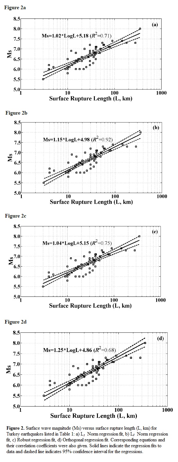
Although the choice of confidence coefficient is somewhat arbitrary, in practice 90%, 95%, and 99% intervals are often used, with 95 % being the most commonly used. So, confidence interval limits of each regression relation used in this study were calculated for 90%, 95%, and 99% confidence interval and these values were given in Table 2 in detailed. These confidence intervals are designed to estimate statistical characteristics of sampled data. However, confidence intervals are more flexible and can be used practically in more situations. Confidence interval generates a lower and upper limit and these limits define the most probable concentration range in which the true parameter ought to lie. The interval estimate also gives an indication of how much uncertainty there is in the estimate of the true value. For this study, there are reliable surface wave magnitudes and rupture lengths in the instrumental period for 63 earthquakes as given in Table 1. From the regression analyses, L₂ Norm and Robust regressions between Ms and Log (L) give a standard deviation of 0.03 in Ms, L₁ Norm and Orthogonal regressions give a standard deviation of 0.04 in Ms, The confidence interval limits computed from given data contains the mean values which is calculated from the regression relations in the Equations 6 to 9. That is, for all lower and upper confidence interval limits (90%, 95% and 99%), as shown in Table 2, these intervals cover the mean values for all regression. Also, the number of earthquakes in 90% confidence limit of the regressions was calculated for each regression and it was found as 14 events for L₂ Norm, 21 events for L₁ Norm, 14 events for Robust and, 17 events for Orthogonal regression. For 99% confidence limit of the regressions, the number of earthquakes was calculated as 25 events for L₂ Norm, 25 events for L₁ Norm, 23 events for Robust and, 29 events for Orthogonal regression.

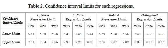
As shown in Figures 2a to 2d, correlation coefficients of these regression fits are nearly the same as L₂ (R²=0.71) Norm and Orthogonal regression (R²=0.68). Correlation coefficient for Robust regression is calculated as 0.75. However, this value is found as R²=0.92 for L₁ Norm and seems quite good. Ms versus L for whole regression methods with fit curves, corresponding equation and 95% confidence interval are given in Figures 2a to 2d. Also, the number of earthquakes for 95% confidence limit of the regressions is calculated in all methods and it is found as 16 events for L₂ Norm, 22 events for L₁ Norm, 20 events for Robust and, 22 events for Orthogonal regression. Thus, the highest number of earthquakes in 95% confidence interval is observed for L₁ Norm and Orthogonal regression.

Regression analysis is routinely used by researchers in many disciplines to fit mathematical models to observed data. Linear least squares estimates can behave badly when the error distribution is not normal, particularly when the errors are heavy-tailed. The traditional estimation technique of least squares is efficient if the error terms are independent of the regressors and are identically and independently distributed as a normal. While the unobserved random disturbances in a regression model are often assumed to be normally distributed, real data are often replete with outliers that lie far from the pattern evidenced by a majority of the data. While these errors may be the result of measurement inaccuracies or human recording error, many outliers are generated by genuinely thick-tailed or asymmetric error distributions. In such cases, discarding outliers is inappropriate since they are representative of the true data generating process (Boyer et al. 2003). The use of any regression criterion is appropriate when it is suspected that a small portion of the data being analyzed is unreliable (i.e., contains data outliers). Regression criterions have the capability of effectively ignoring a few bad data points while emphasizing the majority of data points which more properly reflect the true nature of the data. An insightful and useful characterization of a solution to the problem is to minimize the sum of residual error magnitude. The sum of error magnitudes is of particular use in many applications where the data vector contains a small number of data outliers. In such cases, the sum of squared errors criterion is unduly influenced by these data outliers and thereby often leads to a poor selection of the coefficient vector. The sum of error magnitudes, however, tends to ignore the data outliers provided that they are relatively few in number. In often happens that these data points cluster about a line. As shown in Figures 2a to 2d, four plots of data set provides a visual mechanism for determining the basic nature of the relationships between surface wave magnitude and rupture length. Although the data concentration is between 10 and 100 km and the data does not include outliers, lots of the data remain outside of the confidence limits in all regression fits. However, there are the same values of rupture length for different magnitude values. For example, also can be seen in Table 1, for a rupture length of 30 km there are four different magnitude values such as 6.2, 6.4, 6.8, 6.9 and 7.1 (there are another examples like these values in Table 1). However, all these earthquakes (as seen in Figures 2a to 2d) remained outside the confidence intervals. This means that obtained regressions cannot always reflect the characteristics of earthquakes. As stated above, geological structure has a strong effect on the rupture length. As a result, it is apparent that these regression fits conforms more accurately to the given data points and tends to ignore these data outliers.

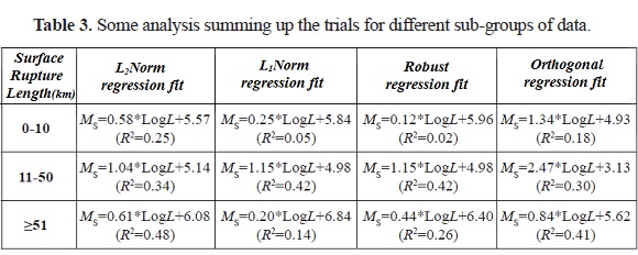
As shown in Figures 2a to 2d, all data interval for rupture lengths is used in the analysis. In order to make a detailed assessment, the earthquakes were grouped into different three sub-groups according to their rupture lengths. All sub-groups and calculations are given in Table 3. In order to obtain the regression relations, the analyses were done for 1 to 10 km, 11 to 50 km, and larger than 51 km. To make a sub-group of rupture lengths, earthquake magnitude level given in Figure 1 were also taken into account. As shown in Figure 1, the earthquakes were grouped into three broad categories: 5.5≤Ms≤6.0 (9 events), 6.1≤Ms≤7.0 (41 events), and Ms≥7.1 (13 events). These magnitude intervals are accordance with the rupture length intervals given above. That is, the earthquakes having 0-10 km (10 events) rupture lengths have the magnitude interval which generally varies from 5.5 to 6.0. Also, the earthquakes having 11-50 km (43 events) rupture lengths have the magnitude interval between 6.1 and 7.0, and the earthquakes having larger than 51 (10 events) km rupture lengths have the magnitude interval higher than 7.1. Thus, the rupture lengths intervals in Table 3 were prepared in properly to the magnitude groups in tectonic map. It can be clearly seen that correlation coefficients in all regressions are rather weak for all sub-groups. These calculated weak coefficients may be result of a small number of data or large scattering of data. Also, these results indicate that subdividing the data set according to various rupture lengths does not greatly improve the statistical significance of the regressions and these regressions may provide more reliable results with the usage of all data set. Thus, the results suggest that separating the earthquakes by their rupture lengths is insignificant for rupture length relationships.

Several empirical relationships between rupture length and magnitude from many different regions around the world including Turkey are proposed by several authors. Acharya (1979) found following equation for 11 earthquakes occurred in Turkey:

Ms = 0.92* LogL + 5.33 (with a correlation coefficient = 0.83) (10)

Wells and Coppersmith (1994) compiled a large dataset consisting of 244 earthquakes from around the world, along with reliable estimates of their source dimensions and moment magnitudes. They developed a series of empirical relationships for fault length, width, area, maximum and average displacement for the whole of their dataset but also separately for each faulting-type group (normal, thrust, strike-slip). They calculated following relation for global earthquakes:

Ms = 1.16* LogL + 5.08 (with a correlation coefficient = 0.89) (11)

Ambraseys and Jackson (1998) proposed following empirical relationship for Eastern Mediterranean earthquakes covering Turkey:

Ms = 1.04* LogL + 5.27 (12)

It is well known that the length of rupture at the surface is related with earthquake magnitude and many studies in literature relate magnitude to rupture length or some another earthquake source parameters for regions of different geographic or tectonic setting (e.g., Acharya, 1979; Wells and Coppersmith, 1994). With developing a regression relationship among magnitude and rupture length, it can be predicted an expected value for a dependent parameter from an observed independent parameter. Independent or dependent parameters will depend on the application, either the expected magnitude for a given rupture length or the expected fault length for a given magnitude. The suggested empirical relationship in this study can be used to assess maximum earthquake magnitude for a particular fault zone or an earthquake source. The assumption that a given magnitude is a maximum value is valid only if the rupture length also is considered a maximum value. Evaluating the segmentation of a fault zone provides a basis for assessing the maximum length of future ruptures. Given that the length and magnitude are assessed to be maximum values, empirical relations between magnitude and rupture length will provide the expected maximum magnitudes. These are expected maximum magnitudes for the given maximum fault lengths. Thus, it can be concluded that rupture length regressions presented here are appropriate for estimating magnitudes for expected ruptures along the related fault segments. Applying rupture length relations to estimating magnitudes may help to overcome uncertainties associated with estimating the surface rupture length for some seismic sources (Wells and Coppersmith, 1994). Also, for engineering estimation purposes, Acharya (1979) stated that the use of mean magnitude in magnitude rupture-length relationship should be sufficient since there is considerable evidence that beyond certain earthquake magnitude.

Consequently, a comparison of the empirical relationships is made between magnitude and rupture length considering the correlation coefficients. As stated above, the correlation coefficient and the number of events in confidence limit of L₁ Norm regression is the highest among the others. This value is very close to 1.0 and this means that it provides more quantitative assessment of fit than the other L₂, Robust and Orthogonal regression. As a result, it can be suggested that Equation (7) is more suitable empirical relationship between surface wave magnitude and surface rupture length for earthquakes occurred in and around Turkey. Also, the predictive relationship between magnitude and rupture length for the instrumental period is almost identical to those derived by different authors for Turkey earthquakes.

Conclusions

In this study, an application of different statistical regression methods is made and it is discussed how can be decided for the selection of the best regression method for a given data set. Then, a linear relationship between the surface wave magnitude (Ms) and rupture lengths (L) is derived for Turkey earthquakes. For this purpose, the earthquakes which are in the time interval between 1905 and 2005 and whose magnitudes are greater than 5.5 are used. In the analyses, there are 63 great earthquakes whose magnitude ranges vary from 5.5 to 8.0 and rupture length changes between 3 and 350 km. In order to estimate the best empirical relationship from different statistical models, four regression norms are used as (i) Least Squares, (ii) Least Sum of Absolute Deviations, (iii) Total Least Squares or Orthogonal and, (iv) Robust Regression. In order to identify the quality of the fit in a linear regression and to select the most suitable empirical relationship for data set, the correlation coefficient (R²) as a quite simple and very practicable tool is used.

The present research has confirmed a clear and straightforward relationship between magnitude (Ms), the surface rupture length (L) for Turkey earthquakes. There is not a general equation between Ms and L for Turkey earthquakes and only a few authors suggested different relationships for different parts of Turkey. In order to obtain more appropriate and reliable empirical relationship between magnitude and the surface rupture length of Turkey earthquakes, log-linear scale is used in four different regressions and different equations are derived. As a result, the relationship calculated as Ms = 1.15* LogL + 4.98 with a strong correlation coefficient R²=0.92 given by L₁ Norm is suggested for Turkey earthquakes.

Acknowledgments

The author would like to thank to Professor Dr. Hakan KARSLI for his helps in preparing the analysis codes and anonymous reviewers for their useful and constructive suggestions in improving this paper. Also, the computer programs used in this study are partially covered by Gumushane University (Turkey) with project no 2012.02.1717.2.

---

References

Abdelkader, G., Ali, L., & Rachida, R., (2010). Robust nonparametric estimation for spatial regression, Journal of Statistical Planning and Inference, 140, 1656-1670.

Acharya, H.K., (1979). Regional variations in the rupture-length magnitude relationships and their dynamical significance, Bulletin of the Seismological Society of America, 69(6), 2063-2084.

Aksari, D., Karabulut, H., & Özalaybey, S., (2010). Stress interactions of three moderate size earthquakes in Afyon, southwestern Turkey, Tectonophysics, 485, 141-153.

Aktar, M., Ergin, M., Ozalaybey, S., Tapirdamaz, C., Yörük, A., & Bicmen, F., (2000). A lower crustal event in the northeast Mediterranean: The 1998 Adana earthquake (Mw=6.2) and its aftershocks., Geophys. Res. Lett., 27, 2361–2364.

Akyüz, H.S., Hartleb, R., Barka, A., Altunel, E., Sunal, G., Meyer, B.,& Armijo, R., (2002). Surface Rupture and Slip Distribution of the 12 November 1999 Düzce earthquake (M 7.1), North Anatolian Fault, Bolu, Turkey, Bulletin of the Seismological Society of America 92(1), 61-66.

Alptekin, Ö., Nábĕlek, J.L., & Toksöz, M.N., (1998). Source mechanism of the Bartin earthquake of September 3, 1968 in northwestern Turkey: Evidence for active thrust faulting at the southern Black Sea margin, Tectonophysics, 122(1–2), 73–88.

Ambraseys, N.N., & Zatopek, S. (1969). The Mudurnu Valley, West Anatolia, Turkey, earthquake of 22 July 1967, Bulletin of the Seismological Society of America, 59(2), 521-589.

Ambraseys, N.N., & Tchalenko, J.S., (1972). Seismotectonic aspects of the Gediz, Turkey, earthquake of March 1970, Geophys. J. R. Astron. Soc., 30, 229-252.

Ambraseys, N.N., (1978). Middle East-A reappraisal of the seismicity, Engineering Geology, 11, 19-32.

Ambraseys, N.N., & Jackson J.A., (1998). Faulting associated with historical and recent earthquakes in the Mediterranean region, Geophysics Journal International, 133, 390-406.

Ambraseys, N.N., & Jackson, J.A., (2000). Seismicity of the Sea of Marmara (Turkey) since 1500, Geophysics Journal International, 141, F1-F6.

Barka, A., Akyuz, H.S., Altunel, E., Sunal, G., Cakir, Z., Dikbas, A., Yerli, B., Armijo, R., Meyer, B., Chabalier, J.B.de., Rockwell, T., Dolan, J.R., Hartleb, R., Dawson, T., Christofferson, S., Tucker, A., Fumal, T., Langridge, R., Stenner, H., Lettis, W., Bachhuber, J., & Page, W., (2002). The Surface Rupture and Slip Distribution of the 17 August 1999 İzmit Earthquake (M 7.4), North Anatolian Fault, Bulletin of the Seismological Society of America, 92(1), 43-60.

Benetatos, C., Kiratzi, A., Ganas, A., Ziazia, M., Plessa, A., & Drakatos, G., (2006). Strike-slip motions in the Gulf of Siğaçik (western Turkey): Properties of the 17 October 2005 earthquake seismic sequence, Tectonophysics, 426, 263–279.

Boyer, B.H., McDonald, J.B., & Newey, W.K., (2003). A comparison of partially adaptive and reweighted least squares estimation, Econometric Reviews, 115–134.

Bozkurt, E., 2001. Neotectonics of Turkey-a synthesis, Geodinamica Acta, 14, 3-30.

Brunbaugh, D.S & Pınar, A., (2001). Preliminary Results of Study of the Mechanism of the December 26,1939 Erzincan Earthquake (M=7.9), American Geophysical Union, Fall Meeting 2001, abstract #S52E-0690.

Cadzow, J.A., (2002). Minimum ℓ1, ℓ2 and ℓ∞ norm approximate solutions to an overdetermined system of linear equations, Digital Signal Processing, 12, 524-560.

Carrol, R.J., & Ruppert, D., (1996). The use and misuse of orthogonal regression estimation in linear errors-in-variables models, The American Statistician, 50, 1-6.

Dewey, J.W., (1976). Seismicity of northern Anatolia, Bulletin of the Seismological Society of America, 66(3), 843-868.

Eyidoğan, H., & Jackson, J.A., (1985). Seismological Study of Normal Faulting in the Demirci, Alaşehir and Gediz earthquakes of 1969-70 in western Turkey: Implications for the nature and geometry of deformation in the continental crust, Geophysical Journal of the Royal Astronomical Society, 81, 569-607.

Eyidoğan, H., Nalbant, S.S., Barka, A., & King, G.J.P., 1999. Static stress changes induced by the 1924 Pasinler (M=6.8) and 1983 Horosan-Narman (M=6.8) Earthquakes, Northeastern Turkey, Terra Nova, 11(1), 38-44.

Fuenzalida, H., Dorbath, L., Cisternas, A., Eyidoğan, H., Barka, A., Rivera, L., Haessler, H., Philip, H., & Lyberis, N., (1997). Mechanism of the 1992 Erzincan earthquake and its aftershocks, tectonics of the Erzincan Basin and decoupling on the North Anatolian Fault, Geophys. J. Int., 129, 1-28.

Giloni, A., & Padberg, M., (2002). Alternative methods of linear regression, Mathematical and Computer Modeling, 35, 361-374.

Giloni, A, Simonoff, J.S., & Sengupta, B., (2006). Robust weighted LAD regression, Computational Statistics and Data Analysis, 50, 3124-3140.

Grosser, H., Baumbach, M., Berckhemer, H., Baier, B., Karahan, A., Schelle, H., Krüger, F., Paulat, A., Michel, G., Demirtas, R., Gencoglu, S., & Yılmaz, R., (1998). The Erzincan (Turkey) earthquake (Ms 6.8) of March 13, 1992, and its aftershock sequence, Pure Applied Geophysics, 152, 465-505.

Hanks, T.C., & Kanamori, H., (1979). A moment magnitude scale, Journal of Geophysical Research, 85, 2348-2350.

Hearn, H.E., Hager, B.H., & Reilinger, R.E., 2002. Viscoelastic deformation from North Anatolian Fault Zone earthquakes and the eastern Mediterranean GPS velocity field, Geophysical Research Letters, 29, 10.1029/2002GL014889, X-1, X-3.

Heo, J.H., Kho, Y.W., Shin, H., Kim, S., & Kim, T., (2008). Regression equations of probability plot correlation coefficient test statistics from several probability distributions, Journal of Hydrology, 355, 1-15.

Huber, P.J., (1964). Robust estimation of a location parameter, Annals of Mathematical Statistics, 35, 73-101.

Huber, P.J., 1981. Robust Statistics, 2nd edn, pp. 354, Wiley, NewYork.

Huber, P.J., (1987). The place of the L₁ norm in robust estimation, In: Dodge, Y. (Ed.), Statistical data analysis based on the L₁ norm and related methods, North-Holland, Amsterdam, 23-33 pp.

Irmak, T.S., (2000). The source-rupture processes of recent large Turkey earthquakes, Individual Studies, International Institute of Seismology and Earthquake Engineering, 36, 131-143.

Lekkas, E., & Vassilakis, E., (1999). Adana Earthquake: Peculiar damage distribution and seismotectonic characteristics, Advances in Earthquake Engineering, Earthquake Resistant Engineering Structures, 4, 785-798.

Leng, L., Zhang, T., Kleinman, L., & Zhu, W., (2007). Ordinary Least Square Regression, Orthogonal Regression, Geometric Mean Regression and their Applications in Aerosol Science, Journal of Physics, Conference Series, 78, doi:10.1088/1742-6596/78/1/012084.

Maronna, R., (2005). Principal components and orthogonal regression based on robust scales, Technometrics, 47, 264-273.

McKenzie, D.P., (1972). Active tectonics of the Mediterranean region, Geophys. J. R. Astron. Soc., 30, 109-185.

Milkereit, C., Grosser, H., Wang, R., Wetzel, H.U., Woith, H., Karakisa, S., Zünbül, S., & Zschau, J., (2004). Implications of the 2003 Bingöl Earthquake for the interaction between the North and East Anatolian faults, Bulletin of the Seismological Society of America, 94(6), 2400-2406.

Moazami-Goudarzi, K., & Akasheh, B., (1977). The earthquake of September 6, 1975 in Lice (eastern Turkey), Tectonophysics, 40, 361-368.

Nalbant, S.S., Hubert, A., & King, G.J.P., (1998). Stress coupling between earthquakes in northwest Turkey and the North Aegean Sea, Journal of Geophysical Research, 103, 24469-24486.

Nalbant, S., Mcclokey, J., Steacy, S., & Barka, A., (2002). Stress accumulation and increased seismic risk in eastern Turkey, Earth and Planet Science Letters, 195, 291-298.

Ozener, H., Arpat, E., Ergintav, S., Dogru, A., Cakmak., R., Turgut, B., Dogan, U., (2010). Kinematics of the eastern part of the North Anatolian Fault Zone, Journal of Geodynamics, 49, 141–150.

Pavlides, S., & Caputo, R., (2004). Magnitude versus faults' surface parameters: quantitative relationships from the Aegean region, Tectonophysics 380, 159-188.

Pınar, A., (1998). Source inversion of the October 1, 1995 Dinar earthquake (Ms=6.1): a rupture model with implications for seismotectonics in SW Turkey, Tectonophysics, 292, 255-266.

Ritsema, A.R., (1974). The earthquake mechanism of the Balkan region, Sci. Rep. 74-4, pp. 1-36, R. Neth. Meteorol. Inst., De Bilt.

Rousseeuw, R.J., & Leroy, A.M., (1987). Robust Regression and Outlier Detection, Wiley, New York 329 pp.

Shi, M., & Lukas, M.A., (2005). Sensitivity analysis of constrained linear L₁ regression: perturbations to response and predictor variables, Computational Statistics and Data Analysis, 48, 779-802.

Sinha, S.K., Field, C.A., & Smith, B., (2003). Robust estimation of nonlinear regression with autoregressive errors, Statistics and Probability Letters, 63, 49-59.

Şaroğlu, F., Emre, O., & Kuşcu, I., 1992. Active fault map of Turkey, General Directorate of Mineral Research and Exploration, Ankara, Turkey.

Şentürk, D., & Nguyen, D.V., (2006). Estimation in covariate-adjusted regression, Computational Statistics and Data Analysis, 50, 3294-3310.

Taymaz, T., Jackson, J., & McKenzie, D., (1991). Active tectonics of the north and central Aegean Sea, Geophys. J. Int., 106, 433-490.

Tibi, R., Bock, G., Xia, Y., Baumbach, M., Grosser H., Milkereit, C., Karakisa, S., Zünbül S., Kind, R., & Zschau, J., (2001). Rupture processes of the 1999 August 17 Izmit and November 12 Düzce (Turkey) earthquakes, Geophys. J. Int., 144, F1-F7.

Turgut, A., (2007). Investigation of the relationship between depth of focus and overburden and the surface ruptures related with strike slip faults by mechanical models, MSc Thesis, Hacettepe University, Ankara, Turkey (in Turkish with English abstract).

Ulusay, R., Tuncay, E., Sönmez, E., & Gökçeoğlu, C., 2004. An attenuation relationship based on Turkish strong motion data and iso-acceleration map of Turkey, Engineering Geology, 74, 264-291.

Weisberg, S., (1985). Applied Linear Regression, 2nd edn, John Wiley and Sons, New York, 310 pp.

Wells, D., & Coppersmith, J.K., (1994). New empirical relationships among magnitude, rupture length, rupture width, rupture area, and surface displacement, Bulletin of the Seismological Society of America, 84(4), 974-1002.

Westaway, R., (1990). Block rotation in western Turkey, 1, Observational evidence, J. Geophys. Res., 95, 19857-19884.

Yalcinkaya, E., (2005), Stochastic finite-fault modeling of ground motions from the June 27, 1998 Adana-Ceyhan earthquake, Earth Planets Space, 57, 107-115.