Validating the University of Delaware’s precipitation and temperature database for northern South America

Vast sections of the planet face either a dearth of ground-based weather stations or are hampered by the poor quality of those in service. In response, researchers are forced to turn to climate field databases, as they constitute a source of reliable information for local studies. Insofar as the Amazon region, these databases prove to be valuable given their open-access platform and the fact that this expansive region possesses few quality stations (coupled with insufficient temporal coverage). However, before basing research on such archives, this information should be compared against in situ station measurements. Then, the present study assesses the validity of temperature and precipitation information furnished by University of Delaware’s database (UD-ATP) by means of a comparison with the open-access information available from Climate Explorer project (CLIMEXP). Results show that UD-ATP database offers better precipitation data representation, especially on Brazil, which is perhaps the effect of higher-quality and larger-quantity observed data.

DOI: https://doi.org/10.15446/dyna.v82n194.46160

Validación de la precipitación y temperatura de la base de datos de la Universidad de Delaware en el norte de Suramérica

Juan Sebastián Fontalvo-García ^a, José David Santos-Gómez ^{a, b} & Juan Diego Giraldo-Osorio ^a

^a Facultad de Ingeniería, Pontificia Universidad Javeriana, Bogotá, Colombia. fontalvoj@javeriana.edu.co, j.giraldoo@javeriana.edu.co
^b Facultad de Ingeniería, Universidad de los Andes, Bogotá, Colombia. jd.santos10@uniandes.edu.co

Received: October 14^th, 2014. Received in revised form: July 29^th, 2015. Accepted: August 4^th, 2015.

This work is licensed under a Creative Commons Attribution-NonCommercial-NoDerivatives 4.0 International License.

---

Abstract
Vast sections of the planet face either a dearth of ground-based weather stations or are hampered by the poor quality of those in service. In response, researchers are forced to turn to climate field databases, as they constitute a source of reliable information for local studies. Insofar as the Amazon region, these databases prove to be valuable given their open-access platform and the fact that this expansive region possesses few quality stations (coupled with insufficient temporal coverage). However, before basing research on such archives, this information should be compared against in situ station measurements. Then, the present study assesses the validity of temperature and precipitation information furnished by University of Delaware's database (UD-ATP) by means of a comparison with the open-access information available from Climate Explorer project (CLIMEXP). Results show that UD-ATP database offers better precipitation data representation, especially on Brazil, which is perhaps the effect of higher-quality and larger-quantity observed data.

Keywords: time series of interpolated climate fields; precipitation; temperature; South America; Amazon region.

Resumen
Debido a la carencia de estaciones en tierra, o a la mala calidad de éstas, en amplias regiones del planeta, las bases de datos de campos climáticos emergen como fuentes de información confiable para realizar estudios locales. En el caso específico de la Amazonía, estas bases de datos son valiosas porque son de libre acceso, y porque este vasto territorio cuenta con pocas estaciones de calidad y suficiente longitud. Sin embargo, previo a su utilización, es necesario comparar estos datos con la información disponible de las estaciones. Se verificó la validez de la información de precipitación y temperatura contenida en la base de datos de la Universidad de Delaware (UD-ATP), contrastándola con la información de libre acceso disponible en el Climate Explorer (CLIMEXP). Se encontró que la precipitación es mejor representada por la base de datos UD-ATP, y que los resultados son mejores sobre el territorio brasilero, posiblemente por la mejor calidad de los registros observados.

Palabras clave: Series temporales de campos climáticos interpolados; precipitación; temperatura; Suramérica; región de la Amazonía.

---

1. Introduction

For regions as massive as the one occupied by the Amazon Rainforest, climate variables are notorious for being incomplete, fragmented and outdated. Together, these inconveniences comprise the primary limitations faced by climatologists. In general, meteorological station data for the Amazon is not uniform in spatial or temporal terms. The construction of evenly distributed grids is crucial to climate analysis, seeing as these are the principal sources for variables in regions removed from measuring stations; in addition, they facilitate local studies in inaccessible regions which lacking information [1-3]. Disciplines benefitting from these interpolated grids are as diverse as: agriculture, biological sciences, hydrology, water resources management, and climate change studies [1,4-6].

On a global scale, high-resolution fields of climate variables are found for long-term monthly averages. For example, Hijmans et al. [4] built monthly average grids for the years 1950-2000 that take into account precipitation and temperature with 30" (~1 km) spatial resolution; New et al. [5] laid out monthly averages for eight climate variables and a wide range of statistics extracted from data for 1960-1990 with 10' (~20 km) spatial resolution. Yet, while time series have been constructed to cover the entire planet, spatial resolution has turned out to be much harder to achieve, possibly due to the spatial and temporal gaps plaguing the data. For the most part, global databases rely on interpolation with a spatial resolution of 0.5° (~50 km); one of the most well-known is that developed by the Climate Research Unit (CRU) at the University of East Anglia, most recently updated to encompass the period spanning 1900-2012 [6-8]. These climate field time-series databases often stem from the direct interpolation of station data, which grants the highest spatial resolution and greatest length of time [9-11]. Likewise, there is the inclusion of satellite-based observations to assist in the process of interpolation, providing information ranging from 1970 to today [12]. Another method is the reanalysis of observed data in climate models, although this method only covers relatively short periods [13-15].

Nevertheless, interpolated climate-variable maps for specific areas are assembled with extremely high spatio-temporal resolution. From these sets of quasi-continental databases, we highlight the work of (i) Jeffrey et al. [16] for Australia, which depicts precipitation, maximum and minimum temperature, evaporation, solar radiation and vapor pressure information all at 10' spatial resolution, and daily temporal resolution (1890-2000 or 1957-2000, depending on the variable in question); (ii) interpolated precipitation and temperature grids constructed for Europe on a daily basis (1950-2006) at 25 km spatial resolution [1]; (iii) the precipitation and temperature database built by Hutchinson et al. [17] for Canada on a daily basis (1961-2003), and 5' spatial resolution. Database resolution can be even better, at least in spatial terms, when the study is restricted to a smaller area and the information required to carry out the interpolation is of high quality: Perry and Hollys [18] built monthly fields (1961-2000) for 36 variables for the United Kingdom, with 5 km spatial resolution. In the case of Spain, Herrera et al. [19] made daily precipitation and temperature fields (1950-2003) with a spatial resolution of close to 20 km. Additionally, Hurtado-Montoya and Mesa-Sánchez [20] provide invaluable information for Latin America, insofar as it provides monthly historical precipitation grids for Colombia with high spatial resolution by virtue of an optimal integration of updated information and distributed grids (satellite images and re-analysis). Here, the downside is that the interpolated period only runs from 1975 to 2006, and, at the time of writing the present document, restrictions regarding access to this information were in effect.

Ground station information for the Amazon region, located in the northern part of South America is not complete. Most stations in the territory are concentrated in the mountainous region of the Andes range, or near the Brazilian coast. In effect, this concentration leaves large tracts of open jungle plains void of either quality information or with sufficient temporal length. As a way of tackling this information scarcity, researchers look to interpolated databases. Precisely here is where databases like the University of Delaware's Air Temperature and Precipitation database (UD-ATP) comes into play. The database's key features include: open access, more than 100 years of information from across the entire planet with 0.5° spatial resolution, and monthly temporal resolution. Database assessment is indispensable, and the present study has taken on this task, through the validation of UD-ATP precipitation and temperature variable for northern South America. For the purposes of the present study, validation means comparing the UD-ATP data to ground station data obtained via the Climate Explorer (CLIMEXP) webpage using a set of statistical analyses (the Pearson correlation coefficient -R-; and the Kolmogorov-Smirnov -KS- test), in order to verify the fit of probability distributions from station-collected data to those of interpolated grids. Finally, annual cycles from observed data against interpolated grid data were compared, using the normalized root-mean-square error (NRMSE).

2. Study area and data

2.1. Study area

The study area spans 20ºS to 15ºN and 85ºW to 35ºW (see Fig. 1), which corresponds to the northern portion of South America, where the Amazon basin is located. For this region, the CLIMEXP ground-station data, and precipitation and temperature grids from the UD-ATP database, were employed.

2.2. UD-ATP interpolated grids

The UD-ATP information consists of monthly grids of total precipitation and average temperature values for 1901 to 2010 (version V3.01), with 0.5º spatial resolution (approximately 50 km close to the equator) and grid-points centered at 0.25º. These archives encompass all emerged surfaces on Earth (read: dry land areas), relying on 720 x 360 x 1332 pixilation.

The interpolation process, as it pertains to the construction of monthly fields, is explained by Matsuura and Willmott [10,11]. In broad terms, their study collects a myriad of pieces of data from the ground stations that form part of the Global Historical Climatology Network (GHCN2) and gleans data from local agencies supporting the project.

2.3. Climate Explorer (CLIMEXP) ground stations

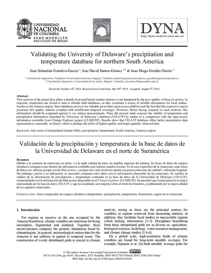
The ground-based data utilized for this study's comparison of grid data come from the CIMEXP (CLIMEXP; [21]), which belongs to the Koninklijk Nederlands Meteorologisch Instituut (KNMI; known in English as the Royal Netherlands Meteorological Institute). Without any sort of financial expectation, CLIMEXP gathers precipitation and temperature variables, among others. The provenance of these variables is global, in line with the project's goal of sharing this invaluable information globally and free of charge. The webpage was selected because it contains current research and boasts the most precipitation and temperature weather stations with monthly registries in the study area. Ground-based station location and record length can be observed in Fig. 2. It is important to bear in mind that the record length is that reported on CLIMEXP, without removing years missing registry data. This situation was seen to occur with some frequency.

3. Preliminary data treatment

3.1. Trimming the UD-ATP interpolated grid

Interpolated grids provide information for the entire planet with 0.5º spatial resolution. In order to trim the grid down for the appropriate study area, NCO (netCDF Operators; [22]) commands were utilized. This procedure creates an archive with nothing more than the data pertaining to the study area. Once the archive was fine-tuned, R software, in tandem with a number of support libraries (notably, the library ncdf makes it easier to manage netcdf files; [23]), allowed us to verify the proper selection of information. As seen in Fig. 1., average yearly (multi-year) precipitation and temperature maps were developed based on time series for monthly interpolated grids from the UD-ATP.

3.2. Selecting and filling gaps in CLIMEXP data

The CLIMEXP registry possesses a variety of in situ measurement stations located across Earth. In order to focus the validation procedure on the study zone, the stations within the aforementioned area were extracted from the CLIMEXP database. Fig. 2 includes maps representing where precipitation and temperature data information are found in the region, showing not only the temporal irregularity of the registries, but also that of the spatial coverage of the stations.

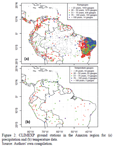
In the relevant study area, we identified 3979 rain gauges. Of these, not all were deemed appropriate for analysis, given that some stations do not meet the criteria established for this study. With regard to these criteria for station selection, the first criterion is of a temporal nature: all those dating back less than 25 years were discarded. It is worth mentioning that great care was taken to fill the missing data for years with gaps of 3 months or less, as per the normal ratio method described by Subramanya ([24], p. 26). Nonetheless, it was quite common to stumble across completely data-free years, a fact which ineluctably forced us to opt for either trimming or abandoning certain time series. The second criterion was geographic: for interpolated grids with 50x50 km² pixels size, each one suffers from high variability in terms of precipitation and temperature data, especially in mountainous regions. In the case of precipitation, those pixels with at least two ground-based measurement stations were employed. A grand total of 280 precipitation stations spread out over 105 pixels in the study zone were chosen, and temporal coverage runs from 25 to 80 years. Fig. 3(a) portrays the spatial location of the selected pixels along with their temporal registry. Readers are reminded that the amount of time in the figure implies that all stations within the pixel report complete data for the same temporal window.

Having outlined the precipitation station selection process, our attention turned to temperature stations. There is a noticeable lack of quantity-not to mention quality-with respect to this aspect. So, to discern the best data sites from the 210 stations found (as compared to 3979 for precipitation) within the study area, less stringent requirements were enforced. Only one temperature station within each pixel was chosen, and the temporal registries start at a minimum of 17 years. In this way, 87 temperature stations provide the relevant data, spread throughout the same number of pixels, with temporal spans from 17 to 110 years. 3(b) shows the results of this search, plus each pixel's temporal registry.

To fill missing precipitation data for the CLIMEXP series within each pixel, the previously mentioned normal ratio method was employed, as expressed by the equation below [24]:

where

= Missing precipitation for month Y in problem station x.
= Yearly average precipitation (multi-year) for problematic station x.
= Yearly average precipitation (multi-year) for n support stations.
= Precipitation/temperature during month Y for n support stations.

This method establishes the neighbor relations among stations located near one another in order to fill out the missing data. For this study "near" was taken to signify that the problem and all support stations fall within the same pixel. Each station was then equally weighted as part of the calculation of missing values.

4. Methodology and results

To reiterate, this paper verifies the UD-ATP interpolated grid data by comparing said dataset with the ground-based weather stations reported in CLIMEXP. With an eye towards ensuring the independence hypothesis of the data, in-situ station data were averaged on a monthly basis for all CLIMEXP stations inside each pixel, resulting in two time series for each pixel studied. While the first time series represents the average of station data, the second represents the UD-ATP grid data in each pixel. Finally, both series were trimmed using the same time window.

An example of the time series obtained for each pixel (analyzed in accordance with the procedure outlined in the previous section) is presented in Fig. 4, with the center placed at 76°15'W-3°15'N. From here on out, this pixel will be discussed as the "pixel-example." This "pixel-example" encompasses part of Southwest Colombia, ranging in elevation from 950 m above mean sea level (amsl; the Cauca River Valley) to 4250 m amsl (the peaks of the Central Colombian Andes), close to the Huila Summit. The pixel's center, however, is situated at roughly 1050 m amsl.

For rainfall, three gauge stations were counted on to arrive at the series for observed data (between 1953 and 1989); however, for temperature, there was only one reliable station (1951-2010). The dispersion diagram included in Fig. 4(d) evinces a systematic positive deviation from the interpolated temperature grids when compared to the station data. Nevertheless, this deviation is not seen in the pixel's constructed precipitation series (Fig. 4c).

To objectively measure the deviations between observed and UD-ATP series, a handful of analytical tools were used: a) deviation calculation between yearly cycles calculated for each series, b) comparison of empirical probability distributions constructed for both datasets (yearly and seasonally) and c) a correlation test to confirm temporal coherence among the data. All of these steps are explored in further detail below.

4.1. Yearly cycle analysis

Yearly cycle analysis allows us to check whether the UD-ATP adequately mimics the intra-yearly variability of the variables, a situation of particular importance because, for example, temperature abides by seasonal cycles in areas located far from the equator. Yet, for tropical zones, rainfall displays two peaks associated with the Intertropical Convergence Zone (ITCZ) passing over these regions.

Averages for observed and UD-ATP series for each variable and each month, including a 95% confidence interval (95% CI), where computed. Confidence intervals were calculated assuming normality-per Eq. (2)-in spite of the fact that the short registry time span of some pixels potentially complicates this assumption:

where

= Average value of x for each month, calculated with the observed data.
= Normal significance value . If significance is 0.05, then ≈ 1.96.
= Standard deviation for x each month, calculated with the observed data.
n = Number of data used to calculate and .
m = Expected value of x.

Yearly precipitation and temperature cycles can be consulted in Fig. 5 for the pixel-example. As expected, the UD-ATP better reflects the annual rainfall cycle than the annual temperature cycle, reinforcing the systematic deviation of the latter dataset for the UD-ATP database versus its representation by CLIMEXP (observed data).

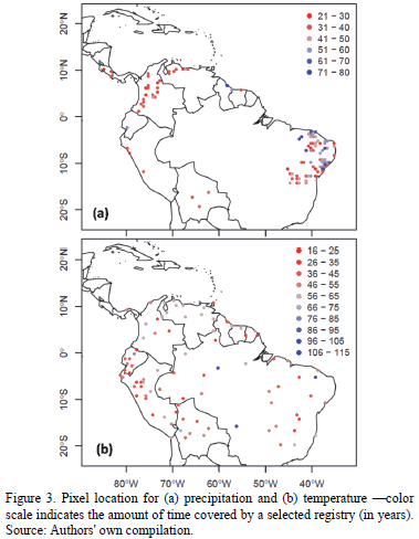
To calculate the degree of deviance between the interpolated and observed yearly cycles, the Mean-Squared Error was used, normalized to fit within the variable's range, which is known as the Normalized Root-Mean-Square Error (NRMSE); the NMRSE helped determine an independent metric of variable magnitude. (i.e. a way to compare deviations in rainy Amazonian regions and arid Peruvian coastal regions, was sought). NRMSE, though, requires the prior calculation of the Root-Mean-Square Error (RMSE; [25]), which is expressed below:

where

= Average variable value for month i, calculated with CLIMEXP data.
= Average variable value for month i, calculated with UD-ATP data.

Completing this step leads us to the NRMSE -Eq. (4)-:

where

x_MAX = Maximum value of monthly average (multi-year) for the variable (i.e. rainiest month of the year or highest average temperature).
x_MIN = Minimum value of monthly average (multi-year) for the variable (i.e. driest month of the year or lowest average temperature).

After computing NRMSE for both variables and all pixels analyzed, the maps shown in Fig. 6 were created. On one hand, precipitation saw the gauges exhibiting the lowest NRMSE clustered in Brazil; for the country, 67 pixels were studied, of which 56 had an NRMSE below 10%. Overall, gauges in other countries performed in a more hit-or-miss fashion: from a group of 38 pixels, only 20 had an NRMSE value less than 10%. But, temperature errors were greater still-only 26 of the 87 pixels possess NRMSE values of less than 10%, with 16 presenting values greater than 100%.

4.2. Goodness-of-fit test for comparing data distribution

The present study employs the Kolmogorov-Smirnov (KS) goodness-of-fit test for two samples. This test allows us to evaluate the fit of any distribution to a dataset by way of comparing the reference's cumulative distribution function (CDF) to the data's empirical CDF. One of the primary benefits of the KS test is that it compares the probability distributions for both datasets without needing to estimate the theoretical distributions for either a priori. It is precisely this strength that makes it well-suited to the present study. The test was used to find out the fit of precipitation and temperature distributions for in situ weather stations (CLIMEXP database taken as reference distribution) and distributions for the same variables in the corresponding pixel using the UD-ATP database.

4.2.1. Computing empirical non-exceedance probabilities

To carry out the KS goodness-of-fit test, empirical non-exceedance probabilities must be assigned to the data (both observed and UD-ATP), ordering them in ascending order. Said probabilities were calculated using probability plotting positioning, which plots yearly time series and estimates a variable's probability of exceeding each value [26], [27]. The general equation reads as follows:

where

P[X<x_i] = Empirical probability of no exceedance for the i-th datum x_i.
i = Data order within the series (ascending).
n = Sample size.
a = Parameter of the plot position, which depends on the distribution to which it will be adjusted.

This study employed Weibull's formula to calculate the non-exceedance probabilities, a formula applicable to any distribution. In this case, a = 0, which in turn translates into a simplified version of Eq. (5):

4.2.2. Goodness-of-fit test p-value

As mentioned above, the KS goodness-of-fit test for two samples is a non-parametric test that assesses the "equality" of two probability functions for two independent samples, determining the maximum distance between the CDF based on the samples. Doing so implies that the precipitation/temperature time series should be obtained from the CLIMEXP database, and those corresponding to the UD-ATP database. The two-tailed KS goodness-of-fit test is as follows:

where

S_m(x), S_n(x) = Empirical CDF of the independent samples calculated with Eq. (6).
m, n = Sample size (even though the present study always saw m=n; inside each pixel, both the CLIMEXP and the UD-ATP series, share the same time span).

It has been shown that asymptotic distribution meets the following standards [28]:

where .

Finally, the p-value of the test is calculated thusly:

Generally speaking, if the p-value is greater than a (the statistical significance level), the null hypothesis is accepted, thus S_m(x) = S_n(x). Well known significance values are 0.01 and 0.05, which are frequently used in several statistical tests.

4.2.3. Results for the goodness-of-fit test

The KS goodness-of-fit test was undertaken for each pixel studied. The time series were split into yearly and seasonal periods, according to seasons occurring in the northern hemisphere: winter (December-January-February); spring (March-April-May); summer (June-July-August); and, autumn (September-October-November). For the sake of clarity, precipitation is defined as the depth of rainfall in each analyzed period (yearly or seasonal), for each year in the registry, while temperature is defined as the average air temperature computed for each analyzed period.

Pixel-example results obtained are visually represented in Fig. 7, where the cumulative empirical probability distributions calculated for precipitation are graphed. The p-value proved to be greater than the significance value (a = 0.05) in every case; this fact leads us to conclude that the distribution of UD-ATP data does indeed adjust to the observed data, though the p-value calculated for temperature in the pixel-example is virtually zero for all tests (not shown), in and of itself an expected situation in light of the previously run tests. Armed with results for each pixel, the maps seen in Fig. 8 were developed; these maps differentiate p-values according to varying significance values (p-value < 0.001 being the worst fit, and p-value > 0.05 indicating that the distributions equal using a good significance value).

Overall, precipitation results were good (see Table 1), even for the Andean region. This implies that the UD-ATP precipitation data reproduces the data observed by ground-based weather stations. Thus, it is possible to rely upon the UD-ATP for areas lacking high-quality data. When looking at the figures, readers should not forget that "summer" was the most deficient season with respect to the number of properly adjusted pixels, which can be chalked up to a concentration of pixels analyzed in Brazilian territory; that is, a territory for which the boreal summer (June-July-August) exhibits low rainfall values. That notwithstanding, the rest of the periods analyzed saw 80% of their pixels well-adjusted, especially true for the Andean countries (Colombia, Ecuador, Peru and Venezuela), where, despite the fact that some pixels have less than stellar performance, the majority have a p-value greater than 0.05. Perhaps this is due to the effect of the Andes on the variables studied. In other words, this geographical feature may cause problems in the interpolation, in addition to the widely recognized precarious nature of weather stations located on mountain ranges.

Temperature, on the other hand, produced poor results (see Fig. 9). As Table 1 evinces, more than half of the pixels had p-values of less than 0.01 for all periods investigated. Though detection of spatial behavior is no easy task with these results, on the whole, the fit for the Amazon Basin and the Brazilian Highlands are better than for the stations located in Andean countries. The latter group ended up demonstrating undesirable adjustments, no doubt attributable to the bulwark known as the Andes Mountain Range, with the concomitant topographical challenges imposed on variable interpolation (mentioned in the previous paragraph). When discussing the results, it is essential to be forthright about the risks of imposing the temperature characterization for a vast area (50x50km²) on only one station. Is very likely that the temperature station is not located close to the pixel center, and if so, it does not represent the temperature variability within the pixel.

4.3. Pearson correlation coefficient

The covariance measures the tandem change of two random variables, which implies that if large values for one of the variables correspond to large values for the other, with the same situation playing out for low values, then covariance is said to be positive. If this is not the case, and low values for one variable match high values for the other, then the covariance is said to be negative. Consequently, covariance indicates the linear relation trend among variables. Nevertheless, sometimes it is hard to explain or interpret the covariance, because it depends on both the magnitude and the units of measurement of the variable. This difficulty can be overcome using the Pearson correlation coefficient (denoted by R) calculated between series. The Pearson correlation coefficient could be interpreted as the normalized version of covariance. The correlation coefficient is distinguished by the fact that it is always comprised between -1 and +1, where +1 is a perfect positive correlation [28].

The project at hand expected, and saw, observed data to be strongly positively correlated to the UD-ATP data (i.e. R values near +1). Furthermore, negative correlations were not expected to be encountered as correlations of this sort would indicate temporal inconsistencies between observed and interpolated grid data. The Pearson correlation results for each pixel can be found in Fig. 10. Both variables have more than 70% of their analyzed pixels with R values above 0.8, but the proportion of pixels for temperature that are poorly correlated (that is, R < 0.5) is smaller than the proportion of the precipitation pixel.

Insofar as the correlation coefficient's spatial distribution, neither variable led to identify any discernible spatial pattern

This conclusion is based on the sprinkling of high and low correlation values from pixel to pixel. This is especially evident for Brazilian pixels in terms of precipitation data.

Colombian-based data for precipitation ranged from adequate to good. Correlations from the northern Peruvian coast provide evidence of an area whose rainfall is difficult to represent for the UD-ATP database. As far as the distribution of the correlation coefficient for temperature is concerned, no overarching spatial behavior stands out, given that low R values are spread throughout the entire study area without regard for a region's topography, whether this is mountainous or open plain.

5. Conclusions

On balance, the UD-ATP database contributes to hydrological research by virtue of its useful information for areas with few reliable ground-based weather stations. However, there are valid concerns about the database's representation of precipitation and temperature variables. Undoubtedly complicated by the nature of measuring these variables, the proper construction of an interpolated grid is sensitive to a number of complex relations inside a geographical zone, especially regional topography (e.g. the Andean mountain range).

The benefits proffered by the UD-ATP really come to the forefront when discussing macro-level hydrological studies, for they cover vast areas with relatively dependable and temporally-adequate information. Its value is amplified when the scientists turn their attention to areas lacking in climate variables, as is the case for much of the Amazon region. However, micro-level studies should be wary of the spatial resolution employed by these databases, which may restrict quality and fail to provide information that is any more worthwhile than that provided by in situ stations (often achieving better spatial interpolation and resolution).

On the whole, UD-ATP precipitation data present better results than temperature, as has been shown throughout the present analysis. The difference in the quality of the two becomes salient from the perspective of yearly cycles, where the interpolated temperature data in many pixels are systematically deviated from the observed data. Not surprisingly, the majority of these deviations popped up around the Andean mountain range.

Results stemming from the goodness-of-fit test reinforce the notion of interpolated precipitation data reliability. Here, pixels for the Andean chain are good, even if they are available in lesser quantity than for the relatively flat regions found in Brazil. The value of such data does not speak for temperature: results for temperature reflect the poor approximation of UD-ATP database for the entire area studied as regards this variable, nowhere more than areas pertaining to mountainous regions.

Cross-correlation analysis led to good results for both variables. Precipitation saw its worst results concentrated in the northern Peruvian coast, a very dry zone, and in Brazilian territory, where result quality fluctuated from pixel to pixel. As has been the case, UD-ATP temperature performance was not strong in this facet. Additionally, it behoves us to point out that spatial distribution does not define any sort of pattern for temperature data.

Lastly, the authors urge that further attention needs to be paid to developing climate databases with high spatial resolution. Such databases are indispensable for the study of areas with strong climate gradients, although we stress the fact that high resolution does not necessarily translate into better data.

Acknowledgments

Interpolated precipitation and air temperature grids from the University of Delaware (UD-ATP) were provided by the National Oceanic and Atmospheric Administration (NOAA) and Office of Oceanic and Atmospheric Research (OAR), as well as the Earth System Research Laboratory (ESRL) and Physical Science Division (PSD) located in Boulder, Colorado, United States of America. This information can be accessed at http://www.esrl.noaa.gov/psd/.

Data of precipitation and air temperature from ground stations were provided by KNMI (Koninklijk Nederlands Meteorologisch Instituut - Royal Netherlands Meteorological Institute) through the Climate Explorer (CLIMEXP) website http://climexp.knmi.nl/.

References

[1] Haylock, M.R., Hofstra, N., Klein-Tank, A.M.G., Klok, E.J., Jones, P.D. and New, M., A European daily high-resolution gridded data set of surface temperature and precipitation for 1950-2006, J. Geophys. Res., 113(D20), pp. D20119, 2008. DOI: 10.1029/2008JD010201.

[2] León-Hernández, J.G., Domínguez-Calle, E.A. y Duque-Nivia, G., Avances más recientes sobre la aplicación de la altimetría radar por satélite en hidrología. Caso de la cuenca amazónica, Ingeniería e Investigación, 28(3), pp. 126-131, 2008.

[3] León-Hernández, J.G., Rubiano-Mejía, J. and Vargas, V., Series temporales de niveles de agua en estaciones virtuales de la Cuenca Amazónica a partir de altimetría radar por satélite, Ingeniería e Investigación, 29(1), pp. 109-114, 2010.

[4] Hijmans, R.J., Cameron, S.E., Parra, J.L., Jones, P.G. and Jarvis, A., Very high resolution interpolated climate surfaces for global land areas, Int. J. Climatol., 25(15), pp. 1965-1978, 2005. DOI: 10.1002/joc.1276.

[5] New, M., Lister, D., Hulme, M. and Makin, I., A high-resolution data set of surface climate over global land areas, Clim. Res., 21(1), pp. 1-25, 2002. DOI: 10.3354/cr021001.

[6] New, M., Hulme, M. and Jones, P., Representing twentieth-century space-time climate variability. Part II: Development of 1901-96 Monthly grids of terrestrial surface climate, J. Climate, 13(13), pp. 2217-2238, 2000. DOI: 10.1175/1520-0442(2000)013<2217:RTCSTC>2.0.CO;2.

[7] Harris, I., Jones, P.D., Osborn, T.J. and Lister, D.H., Updated high-resolution grids of monthly climatic observations - the CRU TS3.10 Dataset, Int. J. Climatol., 34(3), pp. 623-642, 2014. DOI: 10.1002/joc.3711.

[8] Mitchell, T.D. and Jones, P.D., An improved method of constructing a database of monthly climate observations and associated high-resolution grids, Int. J. Climatol., 25(6), pp. 693-712, 2005. DOI: 10.1002/joc.1181.

[9] Fan, Y. and van den Dool, H., A global monthly land surface air temperature analysis for 1948-present, J. Geophys. Res., 113(D1), pp. D01103, 2008, DOI: 10.1029/2007JD008470.

[10] Matsuura, K. and Willmott, C., Terrestrial air temperature: 1900-2010 gridded monthly time series, version V3.01, Global air temperature archive. National Oceanic and Atmospheric Administration (NOAA), Earth System Research Laboratory (ESRL) Physical Science Division (PSD)., [Online]. Jun-2012. [Date of reference July 15^th, 2014] Available at: http://climate.geog.udel.edu/~climate/html_pages/Global2011/README.GlobalTsT2011.html.

[11] Matsuura, K. and Willmott, C., Terrestrial precipitation: 1900-2010 gridded monthly time series, version V3.01, Global precipitation archive. National Oceanic and Atmospheric Administration (NOAA), Earth System Research Laboratory (ESRL) Physical Science Division (PSD)., [Online]. Jun-2012. [Date of reference July 15^th, 2014], Available at: http://climate.geog.udel.edu/~climate/html_pages/Global2011/README.GlobalTsP2011.html.

[12] Adler, R.F., Huffman, G.J., Chang, A., Ferraro, R., Xie, P.-P., Janowiak, J., Rudolf, B., Schneider, U., Curtis, S., Bolvin, D., Gruber, A., Susskind, J., Arkin, P. and Nelkin, E., The version-2 global precipitation climatology project (GPCP) monthly precipitation analysis (1979-Present). J. Hydrometeor, 4(6), pp. 1147-1167, 2003, DOI: 10.1175/1525-7541(2003)004<1147:TVGPCP>2.0.CO;2.

[13] Kalnay, E., Kanamitsu, M., Kistler, R., Collins, W., Deaven, D., Gandin, L., Iredell, M., Saha, S., White, G., Woollen, J., Zhu, Y., Leetmaa, A., Reynolds, R., Chelliah, M., Ebisuzaki, W., Higgins, W., Janowiak, J., Mo, K. C., Ropelewski, C., Wang, J., Jenne, R. and Joseph, D., The NCEP/NCAR 40-Year reanalysis project, Bull. Amer. Meteor. Soc., 77(3), pp. 437-471, 1996. DOI: 10.1175/1520-0477(1996)077<0437:TNYRP>2.0.CO;2.

[14] Xie, P. and Arkin, P.A., Global precipitation: A 17-year monthly analysis based on gauge observations, satellite estimates and numerical model outputs, Bull. Amer. Meteor. Soc., 78(11), pp. 2539-2558, 1997. DOI: 10.1175/1520-0477(1997)078<2539:GPAYMA>2.0.CO;2.

[15] Kanamitsu, M., Ebisuzaki, W., Woollen, J., Yang, S.-K., Hnilo, J.J., Fiorino, M. and Potter, G.L., NCEP-DOE AMIP-II reanalysis (R-2), Bull. Amer. Meteor. Soc., 83(11), pp. 1631-1643, 2002. DOI: 10.1175/BAMS-83-11-1631.

[16] Jeffrey, S.J., Carter, J.O., Moodie, K. B. and Beswick, A.R., Using spatial interpolation to construct a comprehensive archive of Australian climate data, Environmental Modelling & Software, 16(4), pp. 309-330, 2001. DOI: 10.1016/S1364-8152(01)00008-1.

[17] Hutchinson, M.F., McKenney, D.W., Lawrence, K., Pedlar, J. H., Hopkinson, R.F., Milewska, E. and Papadopol, P., Development and testing of Canada-wide interpolated spatial models of daily minimum-maximum temperature and precipitation for 1961-2003, J. Appl. Meteor. Climatol., 48(4), pp. 725-741, 2009. DOI: 10.1175/2008JAMC1979.1.

[18] Perry, M. and Hollis, D., The generation of monthly gridded datasets for a range of climatic variables over the UK, Int. J. Climatol., 25(8), pp. 1041-1054, 2005. DOI: 10.1002/joc.1161.

[19] Herrera, S., Gutiérrez, J.M., Ancell, R., Pons, M.R., Frías, M. D. and Fernández, J., Development and analysis of a 50-year high-resolution daily gridded precipitation dataset over Spain (Spain02), Int. J. Climatol., 32(1), pp. 74-85, 2012, DOI: 10.1002/joc.2256.

[20] Hurtado-Montoya, A.F. and Mesa-Sánchez, Ó.J., Reanalysis of monthly precipitation fields in Colombian territory, DYNA, 81(186), pp. 251-258, 2014. DOI: 10.15446/dyna.v81n186.40419.

[21] van Oldenborgh, G.J., KNMI Climate Explorer, KNMI Climate Explorer, [Online] 1999. [Date of reference July 18^th, 2014], Available at: http://climexp.knmi.nl/.

[22] Zender, C.S., Analysis of self-describing gridded geoscience data with netCDF Operators (NCO), Environmental Modelling & Software, 23(10-11), pp. 1338-1342, 2008. DOI: 10.1016/j.envsoft.2008.03.004.

[23] Pierce, D., ncdf: Interface to Unidata netCDF data files. 2014.

[24] Subramanya, K., Engineering Hydrology, 3^rd edition. Singapore: McGraw-Hill Education, 2009.

[25] Hyndman, R.J. and Koehler, A.B., Another look at measures of forecast accuracy, International Journal of Forecasting, 22(4), pp. 679-688, 2006. DOI: 10.1016/j.ijforecast.2006.03.001.

[26] De, M., A new unbiased plotting position formula for Gumbel distribution, Stochastic Environmental Research and Risk Assessment, 14(1), pp. 1-7, 2000. DOI: 10.1007/s004770050001.

[27] Shabri, A., A Comparison of plotting formulas for the pearson type III distribution, Jurnal Teknologi C, [Online]. 36C, pp. 61-74, 2002, Available at: http://www.penerbit.utm.my/onlinejournal/36/C/JT36C5.pdf.

[28] Gibbons, J.D. and Chakraborti, S., Nonparametric Statistical inference, 5 ed. Boca Raton: Chapman and Hall/CRC, 2010.

J.S. Fontalvo García, BSc. in Civil Engineeringin 2014 from Pontificia Universidad Javeriana, Colombia. Currently studying a MSc. in Civil Engineering at Pontificia Universidad Javeriana., Bogotá, Colombia. ORCID: 0000-0003-1041-8286

J.D. Santos Gómez, BSc. in Civil Engineering in 2014 from Pontificia Universidad Javeriana, Colombia. Currently studying a MSc. in Civil Engineering at Universidad de los Andes, Bogotá, Colombia. ORCID: 0000-0002-9641-3082

J.D. Giraldo Osorio, BSc. in Civil Engineering in 2001 from Universidad Nacional de Colombia, Colombia. Is MSc. in Civil Engineering, in 2003, focused on water resources management, from Universidad de los Andes, Colombia. PhD. in water resources in 2012, from Universidad Politécnica de Cartagena, Spain. He is currently a full professor at the Civil Engineering Department, School of Engineering, Pontificia Universidad Javeriana, Bogotá D.C., Colombia. ORCID: 0000-0001-6205-3341.