Metodología para la selección de modelos hidrodinámicos - Caso de aplicación: variabilidad espacial de la estructura térmica en el embalse tropical Riogrande II, Colombia

Methodology for hydrodynamic model selection. Case study: spatial variability of the thermal structure in the Riogrande II tropical reservoir, Colombia

Este artículo propone una metodología para la selección guiada de un modelo hidrodinámico para el estudio de los procesos físicos en un embalse, fundamentada en criterios cualitativos y cuantitativos, la cual fue aplicada para estudiar la variabilidad espacial de la estructura térmica en el embalse tropical de Riogrande II. La metodología considera tres etapas: i) definición y búsqueda, ii) preselección y iii) selección. Como resultado los modelos DELFT3D y MIKE3 fueron implementados y se compararon los perfiles de temperatura simulados con aquellos medidos entre el 23 y el 27 de marzo de 2010. ELCOM fue definido como modelo de referencia para comparar las series de tiempo de la profundidad media de la termoclina, la profundidad media de la capa de mezcla y su temperatura media. Para apoyar la selección final se utilizó tres estadísticos: i) el índice de concordancia (d1), ii) el MAE y iii) RMSE, cuyos resultados indicaron que el modelo DELFT3D es para este caso la mejor alternativa.

This article presents a methodology for a guided selection of a hydrodynamic model to study physical processes in a reservoir. It is based on both qualitative and quantitative criteria that are applied in order to study the spatial variability of the thermal structure in the Riogrande II tropical reservoir. The method consists of three main stages: i) definition and search, ii) pre-selection, and iii) selection. As a result, the DELFT3D and MIKE3 models were implemented, and the simulated temperature profiles were compared to field data that was collected between March 23rd and 27th, 2010. ELCOM was defined as a reference model, and the time series of the thermocline depth, the mixing layer depth, and its average temperature were compared with the selected models. The final selection was supported by using three different statistical parameters: the index of agreement (d1), the MAE, and the RMSE. The quantitative analysis showed that the DELFT3D model behaves better than MIKE 3.

DOI: https://doi.org/10.15446/dyna.v83n198.50400

Gabriel Betancur-Pérez ^a, Francisco Mauricio Toro-Botero ^a & Andrés Gómez-Giraldo ^a

^a Facultad de Minas, Universidad Nacional de Colombia - Sede Medellín, Medellín, Colombia. gabetancp@unal.edu.co, fmtoro@unal.edu.co, eagomezgi@unal.edu.co

Received: May 04^rd, 2015. Received in revised form: November 20^th, 2015. Accepted: March 30^th, 2016.

---

This work is licensed under a Creative Commons Attribution-NonCommercial-NoDerivatives 4.0 International License.

Abstract
This article presents a methodology for a guided selection of a hydrodynamic model to study physical processes in a reservoir. It is based on both qualitative and quantitative criteria that are applied in order to study the spatial variability of the thermal structure in the Riogrande II tropical reservoir. The method consists of three main stages: i) definition and search, ii) pre-selection, and iii) selection. As a result, the DELFT3D and MIKE3 models were implemented, and the simulated temperature profiles were compared to field data that was collected between March 23^rd and 27^th, 2010. ELCOM was defined as a reference model, and the time series of the thermocline depth, the mixing layer depth, and its average temperature were compared with the selected models. The final selection was supported by using three different statistical parameters: the index of agreement (d₁), the MAE, and the RMSE. The quantitative analysis showed that the DELFT3D model behaves better than MIKE 3.

Keywords: methodology, model selection, three-dimensional hydrodynamic model, tropical reservoir, thermal structure, ELCOM, DELFT3D, MIKE3.

Resumen
Este artículo propone una metodología para la selección guiada de un modelo hidrodinámico para el estudio de los procesos físicos en un embalse, fundamentada en criterios cualitativos y cuantitativos, la cual fue aplicada para estudiar la variabilidad espacial de la estructura térmica en el embalse tropical de Riogrande II. La metodología considera tres etapas: i) definición y búsqueda, ii) preselección y iii) selección. Como resultado los modelos DELFT3D y MIKE3 fueron implementados y se compararon los perfiles de temperatura simulados con aquellos medidos entre el 23 y el 27 de marzo de 2010. ELCOM fue definido como modelo de referencia para comparar las series de tiempo de la profundidad media de la termoclina, la profundidad media de la capa de mezcla y su temperatura media. Para apoyar la selección final se utilizó tres estadísticos: i) el índice de concordancia (d₁), ii) el MAE y iii) RMSE, cuyos resultados indicaron que el modelo DELFT3D es para este caso la mejor alternativa.

Palabras clave: metodología de selección, modelos hidrodinámicos tridimensionales, embalse tropical, estructura térmica, ELCOM, DELFT3D, MIKE 3.

---

1. Introduction

The physical, climatic and hydrological conditions of rivers, lakes, reservoirs, estuaries and coastal zones, cover a complex dynamic of interaction and feedback between parameters of the representative processes. Given the limited information available on atmospheric variables, such as solar radiation, humidity, air temperature, etc., and on the variables associated to the water body itself, such as free surface, flow rate, temperature, salinity, turbidity, conductivity, etc., the use of complex numerical models are required to understand the behavior of these variables and their interactions.

Moreover, the application of hydrodynamic models with one, two, or three dimensions to study the mass transport [1], temperature [2] and salinity variations -in addition to the velocity and circulation patterns [3] in different water bodies and geographic locations- has increased over recent years. However, in many cases the choice of the model to be used for a specific application is not clear, given the number of options available in the market. This makes the selection of the proper model (tool) a topic that needs to be carefully analyzed [4]. Selection of the proper model for a given application is neither simple nor straightforward since there are several factors involved in the process, such as the model accessibility (public, restricted or commercial), the budget available to resolve the problem, the personal involved, the available information to calibrate and validate the model (field measurements of key variables such as temperature, salinity, speed, current, etc.), and the time required to solve the problem.

As such, several authors have presented their views on the selection of a hydrodynamic model, considering topics such as the cost-complexity and the spatial and temporal dimension that are closely related to the phenomenon [5]. However, there is no systematic method that helps the user to make a good selection of a hydrodynamic model.

This article presents a methodology to perform a guided selection of a hydrodynamic model, based on qualitative criteria (multi-objective analysis) and quantitative tools (statistical analysis of model results). To illustrate the methodology, the spatial variability of the tropical reservoir Riogrande II's thermal structure, during a dry season, was defined as the case study.

2. Suggested methodology for model selection

The suggested methodology considers three stages, the first two being of a descriptive and qualitative nature, while the third is quantitative. Fig. 1 shows a flowchart, which is discussed in the following sections.

2.1. Stage I: Problem definition and search for models

During the first stage, the physical problem to be studied must be clearly defined (process definition) in a mathematical sense by writing the equations (usually conservation laws) that describe the phenomenon under consideration. Then, some exploration criteria are defined and a model inventory should be made that must account for the state of the art of available models. Based on the knowledge gained during this search process, the model user defines if the inventory is robust or not. If it is, the model selection process continues to the next stage, if not, the decision maker will reappraise the exploration criteria and start a new search.

2.2. Stage II: Model preselection

In the second stage, it is necessary to define preselection criteria that are more restrictive than those used in the previous stage, and that will be later used to rank the pre-selected models through the implementation of a multi-purpose analysis [6]. Next, it is necessary to perform a sensitivity analysis for the selected multipurpose analysis method in order to assess whether the obtained solution (rank) is robust. If so, a threshold for the number of numerical models to be used in the next stage is defined and the process continues. Otherwise, the preselection criteria should be reevaluated in order to achieve the previously defined threshold.

2.3. Stage III: Model selection

This is the quantitative stage of the suggested methodology and it requires the numerical models that passed the previous stages to be implemented. In this final stage, it is necessary to clearly define the process control variables and select those that are going to be used to compare the results. To perform this stage, a threshold for the model errors (with respect to a pattern that can be another model or a series of field measurements) is defined, and the model's performance is evaluated by using a statistical tool such as the Mean Square Error (MSE), the Root Square Mean Error (RMSE), or the index of agreement (d₁). Each model's performance is quantified according to a pre-defined scale to rank it and to take the decision as to whether a model is selected.

3. Methods and application

3.1. Case of study: Riogrande II tropical reservoir

The Riogrande II reservoir is a multi-purpose (water and energy supply) reservoir located north of Medellín, Colombia, and is located between the coordinates 75°32'W and 75°26'W and 6°33'N and 6°28'N (Fig. 2). The main tributaries are the Chico River (Q_mean = 5m³/s) to the east, the Grande River (Q_mean = 15m³/s) to the north and the Las Animas stream that has a negligible discharge to the south. The maximum water depth is 42.5m near the dam (near point P1 in Fig. 2), and the water storage volume is 240Mm³ at 2270 m.a.s.l.[7]. The intake to the hydroelectric plant and to the water supply plant is located at point QA2 in Fig. 2.

This three-branch canyon valley reservoir, which according to [8] and [9], has a spatial and temporal variable wind field with a daily cycle (shown in Fig. 2. This includes a space and time variable wind field in the numerical models, which is important because it is an internal wave generator that interacts with the river plumes and generates fast vertical mixing [10].

Numerical simulations made by [9], as well as field measurements during different climatological seasons (rainy and dry seasons), suggest that the Grande River water moves in the reservoir like an intrusive plume from its entrance and then splits in the confluence (C in Fig. 2) into two branches. One travels upstream along the Chico River branch, which affects its plume dynamics, and the second travels south to the intake (QA2 in Fig. 2). The dynamics of these two plumes are mainly affected by the climatological seasons and the river´s water temperature [9].

3.2. Field Measurements for model calibration and validation

In order to facilitate the analysis of the model's results, the reservoir was divided into five zones with similar physical behavior that was based on the following field measurements:

• Zone 1: ChicoRiver Branch (RC1 y RC2)
• Zone 2: Confluence (C)
• Zone 3: Grande River Branch (RG)
• Zone 4: Las Animas stream (QA1 y QA2)
• Zone 5: Dam (P1 y P2)

In order to compare the different models' behavior that passed the second stage of the methodology the models' results were compared to those obtained from a field campaign undertaken between March 23^rd and 27^th, 2010. These data are described in the following paragraphs.

3.2.1. Field Measurements

Temperature profiles were measured between March 23^rd and 27^th, 2010 in the control stations shown in Fig. 2. Fig. 3 shows their typical behavior. The records of the reservoir level were used to assess the mass balance of the system that was reproduced by the implemented models.

Previous reservoir simulations [9] indicate that the temperature profiles in station RG are influenced by the Grande River. They consider that there is no well-defined mixing zone such as that shown in RC1 or P1 profiles (Fig. 3).

In the case of the QA2 profile, despite the selective withdrawal influence [8], it is possible that the reservoir shallowness in this area and the Grande River movement from its mouth to the intake introduce a mixing condition that reduces the temperature gradients. It shows a temperature profile similar to that in the RG station. In both cases, further research and field data are required to evaluate and analyze movement of the plumes and their influence on the reservoir's temperature conditions. Further analysis is also necessary to explain the hydraulic control produced by the Grande River on the Chico River branch. This analysis is outside the scope of this article.

3.2.2. The selection of a pattern for comparison

Those models that passed the two qualitative stages of the methodology will be implemented for this case study. In order to quantify their behavior, their simulated temperature profiles will be compared at selected points and zones of the reservoir using measurements and a reference model (in the methodology a comparison with a pattern, measurements, or another calibrated and validated model, is required). In our case study, results from a calibrated and validated model [9] were chosen to take advantage of the high space and time resolution obtained from the model. This was not available from the measurements. The reference model selected was ELCOM [11], developed by the University of Western Australia, which was calibrated for the field campaign during March 23^rd to 27^th, 2010. ELCOM is a model that has been developed and progressively improved to capture the temperature gradients and the thermal structure in estuaries, lakes and reservoirs. ELCOM incorporates a special mixing model to account for the stratification processes [12], and, therefore, constitutes a reference for other models that seek to represent the thermal stratification in lakes and reservoirs.

ELCOM's results were used to extract time series of temperature at the stations indicated in Fig. 2. Based on these time series, the average depth of the mixing layer and the mean thermocline depth was estimated using the methodology proposed by [13]. Additionally, the average temperature of the mixed layer was calculated once the average depth of the mixed layer had been derived. These three variables will be used to test the models' behavior.

3.3. Multi-purpose analysis methods

The implementation of the suggested methodology requires, during the qualitative stages, the use of a multicriteria analysis method to quickly reduce the potentially suitable models' alternatives for this case study. In this project, the ELECTRE IV [14] method was used, because unlike other multicriteria techniques, such as the PROMETHE method [15] or AHP [16], ELECTRE IV does not use weights to perform the classification process. Instead, a table of metrics is used to define the values for each evaluation criteria, and every alternative forms an impact matrix. Two types of sorting are then performed: ascending and descending. Tie breaker rules are applied to finally rank the alternatives [6].

3.4. Statistical tools used for model behavior evaluation

Several techniques for quantitative evaluation of a model's behavior have been widely explored in atmospheric sciences [17]. Their adaptations to the coastal engineering, undertaken by [18] and [19], are the most important contributions to the numerical model behavior analysis. However, the introduction of the index of agreement, undertaken by [20], is a useful tool to compare and analyze the model results. The statistical parameters used in this paper for the model performance evaluation are presented below.

The most used statistical parameter in model behavior analysis is the Root Mean Square Error (RMSE), given by equation (1) as:

where y_i are the reference values, x_i are the model predictions, and N is the number of data of the time series used in the comparison.

A robust measurement of the prediction's precision is the Mean Absolute Error (MAE) because it is not influenced by the time series' extreme values [21]:

A third and fourth statistical parameter used in the study are the indexes of agreement d₁ and d_2, suggested by [20,21] for g = 1 y 2, respectively:

As is the case for the RMSE, the d₂ index is highly influenced by the differences squared when they are large. For this reason, in this paper, only the d₁ index was used to evaluate the models results.

4. Suggested methodology step by step

4.1. Stage I

The problem under study is the space variation of the Riogrande II reservoir's thermal structure that is under the influence of the wind field during the dry climatological season. The time window to compare the models is between March 23^rd and March 27^th, 2010.

The search criteria to obtain the list of potential models to be used to study the stated problem are:

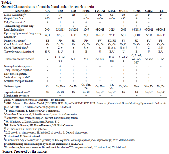
A Three Dimensional Hydrodynamic Model. The interaction that takes place between the different physical processes in a reservoir, such as the time-space variation of the water body temperature under the force of a variable wind field and the dynamics of the river plumes and their interaction makes it necessary to use a 3D hydrodynamic model to correctly approach the stated problem. This makes 1D and 2D models unsuitable. Additionally, the model should have implemented heat fluxes equations with the atmosphere and heat transport in the water body. The turbulent flow of the river plumes in their mixing layer requires an appropriate turbulence closure scheme. A long inventory list of numerical models analyzed in this stage is presented in Table 1.

Sediment transport module: This module was considered because, for future work, this will be a research field. However, no models with sediment transport were implemented in this study and only the hydrodynamics were considered.

4.2. Stage II: Pre-selection

For this stage, the selection criteria were grouped into three categories:

General: Including global characteristics. In this application the following were considered:

• Availability
• Graphical user interface
• Documentation
• Technical support

Flexibility: Configuration options available for the user to properly represent the specific conditions of the phenomenon being considered as well as the representation of the computational domain. In this application, the following were considered:

• Domain horizontal discretization
• Domain Vertical discretization
• Turbulence closure schemes
• Non-hydrostatic module

Heat fluxes: Given the influence these fluxes have on the lake or reservoir's thermal structure, the following were considered:

• Formulae to estimate the latent and sensible heat fluxes
• Transport equation for temperature
• Vertical mixing model

Sediment Transport: This characteristic of the numerical model was considered as an option for future work because the sediment transport process requires a very well defined flow field. The following criteria were considered for the qualitative classification:

• Type of sediment transport process
• Type of sediments
• Bottom morphology evolution

4.2.1. ELECTRE IV method

Once the pre-selection criteria have been defined, the implementation of the ELECTRE IV method follows. To do this, two valuation scales (metrics) were used for the criteria analysis: one with integer numbers between 1 and 10 and a second one with odd numbers between 1 and 9. Using these two metrics, an impact matrix is built with all previously selected criteria. Then, following [14], the reference relationships were estimated by comparing the different alternatives, in groups of two, for each selection criteria. The values that were estimated for the impact matrix and following the preference rules are defined as follows:

• Over Relaxed classification: alternative i OverRelaxed Classifies alternative j if the number of criteria for which alternative i is preferred over alternative j is at least twice the number of criteria alternative j is preferred over alternative i.
• Weak Relaxed classification: alternative iWeakly Relaxed Classifies alternative j if there is at least one criteria by which alternative i is strictly preferred over alternative j and there is no criteria by which alternative j is strictly preferred over alternative i. Also, there is the additional condition that the Strong Over Classification is not satisfied.
• Strong Classification: Alternative i is Strongly Classified over alternative j if there is at least one criteria by which alternative i is strictly preferred over alternative j and there is not a criteria by which alternative j is strictly preferred over alternative i. Also, if the number of criteria by which alternative j is weakly preferred over alternative i is smaller or equal to the number of criteria by which alternative i is preferred (strictly or weakly) over alternative j.

Finally, based on the classifications just defined for each alternative, two lists of alternatives, organized in ascending and descending order are prepared. The final ordered list of alternatives is obtained as the intersection of these two previous lists.

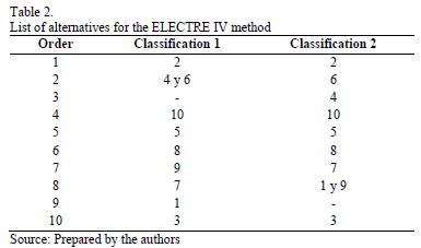
Table 2 shows the final ordered list obtained by following the previously described methodology and for each one of the two previously mentioned evaluation metrics. The numbers appearing in the columns Classification 1 and Classification 2 refer to the model number used in the inventory table (Table 1): alternative 1 refers to the ADCIRC model and alternative 10 refers to the TELEMAC 3D model.

The ELECTRE IV method shows that the DELFT 3D model is the dominant alternative because both classifications placed it in first position on the list. The MIKE 3 and the EFCD 3D models in Classification 1 shared the second position, but in Classification 2, the MIKE3 model only appears in the second position. For this reason, the MIKE3 model was finally classified in the second position. Based on these results, models DELFT 3D and MIKE 3 are chosen for the next stage in the methodology.

4.3. Stage III: Selection

4.3.1. Variables used for comparison

Based on the field measurements and on the time series obtained from the reference model (ELCOM), the variables used to evaluate the behavior of the preselected models are:

• Temperature profiles
• Water level variations in the reservoir
• Mean depth of the mixing layer
• Mean Temperature of the mixing layer
• Mean depth of the thermocline

It is very important that the list of models selected for this stage captures some of the most relevant components of the physical process under study. In this case, the thermal structure of the water body, under the influence of two forcing factors such as the wind field and the river plumes, is well represented by the above-mentioned variables. The depth of the mixing layer and that of the thermocline are important variables because they are a key part of the possible internal waves' appearance in the reservoir [23] as well as being important for its ecological evolution. The mean temperature of the mixing layer is important because it is in this zone that the energy exchange between the water body and the atmosphere occurs [12].

4.3.2. Implementation of the pre-selected models.

DELFT3D is a 3D hydrodynamic model whose governing equations are solved numerically by the Finite Difference technique. The model has been used to simulate flow circulation patterns, heat transport, water quality and bottom morphology under several forcing factors such as wind field and tidal waves with a wide field of applications in coastal zones and estuaries [24]. Since 2010, DELFT3D has been an open code for the hydrodynamic (FLOW), Morphodynamic (MOR), and waves (WAVE) modules. In the year 2013, the water quality module (DELWAQ) was released as an open code. In our application, graphic interphase version 4.00.02 and code 5.00.10.2136 of January 22^nd, 2013 were used for the model implementation of the Riogrande II reservoir.

MIKE3 is the 3D version of the MIKE 21 model developed by the Danish Hydraulic Institute (DHI). It has been widely used in coastal and estuarine applications. The model includes several modules coupled to a graphic interphase. To simulate the thermal structure of the Riogrande II reservoir, the 2012 flexible grid version was used. This version uses the non-structured grid with a finite element discretization in the horizontal plane and a hybrid s - Z coordinate discretization in the vertical plane [25].

Both models were implemented following the reference model (ELCOM) as closely as possible. The reference model was included in this analysis (selection) because it was fully calibrated and validated with field measurements and will be used to generate data not directly available from the measurements. Table 3 shows the general configuration for these three models, in which some differences in the time interval are clear; these are differences due to space discretization. Fig. 4 shows the river discharges and outflows from the reservoir and the atmospheric forcing factors used for all the three models.

4.3.3. Model results and behavior analysis of the models

Error limits

Temperature profiles shown in Fig. 3, typical for tropical zones, differ from those for extra tropical regions. In extra tropical reservoirs typical temperature differences between the surface and bottom of the reservoir may reach values of 20°C [26] with an error of 10% (2°C), which may be reasonable for simulated results. In tropical reservoirs and lakes, the vertical temperature gradients (Figure 3) are much milder than those in extra tropical zones and there are temperature differences between the surface and the bottom in the order of 5°C or 6°C all year long, with a daily cycle. This makes the value of 2°C a very high tolerance error for these cases. By keeping the 10% value for the tolerance error, an equivalent of ± 0.5°C was used in this work as an acceptable limit for the RMSE and MAE errors.

Reservoir free Surface level

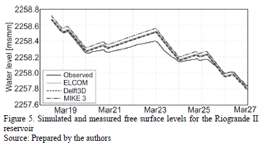
Measured and simulated free surface water levels are shown in Fig. 5. It is clear from the figure that all three models closely follow the measured tendency. The differences found between the measured simulated values, a maximum of 20 cm for March 23^rd, are due to deficiencies in the measured inflows and outflows time series.

The corresponding MAE and RMSE values, that are close to zero (Table 4), indicate the good agreement with measurements. Although, the very similar values obtained for all three models do not allow us to draw any conclusion about which models have a better behavior with respect to this variable. The same behavior can be noticed for the index of agreement, d₁; although, MIKE3 is the one that behaves the poorest. This variable is not good enough for model classification because, as will be shown later, major differences in the parameters are found for the models: differences that are not important for this variable (all models sufficiently capture the free surface water level).

Temperature Profiles

A comparison between simulated and measured temperature profiles is shown in Fig. 6, in which the profiles correspond to those showing the maximum difference between the simulated and computed ones. In zone 1, ELCOM and DELFT3D closely follow the measured profile for which corresponding values for d₁ of 0.93 and 0.91 were found with MAE corresponding values of 0.25°C and 0.30°C. MIKE3 is less precise: in the hypolimnium, the model closely follows the measurements, but as the free water surface is approached the model departs from measurements and even shows an unstable profile. This behavior leads to a d₁ value of 0.83 and an MAE value of 0.48°C (see Fig. 7 and Fig. 8 for more details).

In zone 2, measurements do not show the near surface mixing layer (Fi. 6), which generates a constant temperature vertical gradient that is not sufficiently captured by any model. It instead shows a mixing layer that is about 5m deep. In this zone, ELCOM and DELFT3D produce a d₁ value higher than 0.9 and RMSE values that are smaller than 0.5°C (Fig. 9). MIKE3 shows a value of 0.86 for d₁ and a value of 0.61°C for RMSE.

In zone 3, near the entrance of Grande River, the absence of the surface mixing layer is clear (Fig. 6) and there is a constant temperature vertical gradient. The vertical mixing produced at the river's entrance is responsible for these types of profiles in addition to the wind action in the shallow parts of the reservoir. Values of the index of agreement are presented in Fig. 7, and it is seen that MIKE3 has the smallest values for several profiles in the zone. Analyzing the MAE and RMSE parameters (Figs. 8 and 9), once again MIKE3 has poorer behavior with respect to ELCOM and DELFT3D. Similar behavior is noticed in zone 4 where the effect of the hydro-plant intake is relevant.

Finally, in zone 5, ELCOM and DELFT3D behave in a similar way to in zone 1, with values close to unity for the index of agreement (Fig. 7) and values for the MAE and RMSE that are close to zero (Figs. 8 and 9). In this zone, MIKE3 also has a poorer behavior than the other two models.

These results suggest that the MAE parameter shows better behavioral models. For example, in zone 3 the index of agreement indicates that all three models have poor behavior without being able to differentiate the best one (Fig. 8). The RMSE parameter, on the other hand, demonstrates the better behavior of the ELCOM models, but it is unable to show the differences between DELFT3D and MIKE3. The MAE parameter, however, did show the difference between the three models.

Time series

Three variables of physical interest for the thermal structure of the reservoir are selected for analysis: the thickness of the mixing layer, the mean temperature of this layer, and the depth of the thermocline [13]. The time series of these variables are shown in Fig. 9 for monitoring stations RC1 and QA2.

The thickness of the mixing layer at RC1 (Fig. 10a) is captured by DELFT3D and MIKE3 for the four-day computed period. DELFT3D closely follows the reference model (ELCOM) in both the shape of the series and in the maximum and minimum values. MIKE3, on the other hand, captured the peaks but the shape of the time series looks different from that of the reference model. It showed a constant peak for a period of six hours, which is not in the reference time series. At QA2, both models show more differences with the reference model, although DELFT3D seems to be closer to it. The index of agreement computed for this variable and for several monitoring points in the reservoir is shown in Fig. 8, in which it is clear that DELFT3D better follows the reference model (higher d₁ values than MIKE3).

Time series for the mean temperature of the mixing layer for the monitoring points RC1 and QA2 are shown in Fig. 9b. Mean temperature computed from both models monitoring station RC1 follow the shape of the reference model, but the MIKE3 results are about 0.75°C cooler for the reported period than the reference time series. The ones for DELFT3D are about 0.5°C warmer than the reference time series. For monitoring station QA2, DELFT3D continues with the same behavior, but the temperature difference is now between 1.2°C and 0.5°C warmer. MIKE3 maintains the shape of the daily cycle but is now sometimes warmer and sometimes cooler than the reference. The statistical parameters (d₁, MAE and RMSE) confirm that DELFT3D behaves more similarly to the reference model than MIKE3 does. The behavior of MIKE3 can be explained, with respect to this variable, due to the calibration undertaken to the vertical dispersion coefficient (0.0025). This, for some higher values, produced stable temperature profiles near the surface, resulting in a thicker mixing layer and a deeper thermocline position. For smaller values it generated unstable temperature profiles near the surface with cooler temperature.

This behavior is reflected in the statistical parameters in Fig. 11. The behavior of DELFT3D, generating warmer mean temperatures for the mixing layer, may be related to the parametrization for the heat fluxes included in the model as well as to the wind shear stress on the surface, although a detailed study is needed to confirm this.

Finally, the analysis undertaken to the thermocline depth shows large differences between the reference time series and the computed ones in both monitoring stations (Fig. 10c). It confirms the values of the statistical parameters computed for several stations (Fig. 11). It is important to notice that the methodology the reference model, ELCOM, has implemented a special mixing model differing from those implemented in DELFT3D and MIKE3.

4.3.4. Models classification and final selection

ELCOM was taken as a reference model. The results were used to generate temperature time series that are not available from direct field measurements. This model was not considered for classification purposes due to its proven capacity to simulate thermal stratification and heat fluxes dynamics in lakes and estuaries [23]. It is also widely used to simulate similar cases around the world [27].

Based on the ranges defined by Table 5, the models' performance were estimated for several points in the reservoir zones defined in section 3. Fig. 11 shows that DELFT3D performs better than MIKE3, and its results are similar to ELCOM.

5. Discusion

On the general methodology

The qualitative stages of the methodology are a fundamental part of the selection process because, for practical reasons, it is not possible to implement the long list of available models in the literature. During these stages, it is possible to make a quick review of the alternatives and create a long inventory of possible models that can be used for future work. However, the subjective character of the methods used in these stages may lead to a skewed decision by choosing a model that may not be the best technical option.

This subjective character, which is associated with the definition of the selection criteria and with the implementation of the multi-purpose decision analysis, such as the ELECTRE IV method, may be reduced by looking for methodologies that reduce the subjectivity of the definition of the selection criteria and their evaluation scales. One example is the AHP method [16], which is a technique that involves more than one decision maker and includes a panel of experts that participates in the final decision.

Regarding the quantitative stage of the methodology, the index of agreement for statistical parameters has the advantage over the other two. This is because it is non-dimensional and can be used in a general sense as well as being compared to other models in similar cases. However, care must be taken when using it because it represents a result in a statistical sense. This depends on the set of data used to make comparisons and it is the modeler´s decision to use it instead of the physical results. In this case, the d₁ provides a coherent interpretation of the results and that is why it was selected as the leading parameter for decision-making.

The Statistical parameters

The comparison results showed that the MAE parameter is much more robust, in its physical interpretation, than RMSE, as suggested by [21] and later reported by [28]. In the same sense, the index of agreement is the best parameter to use, given its direct relation to MAE. However, despite the acceptance of this parameter as the leading parameter for selecting and classifying the behavior of hydrodynamic models, there are other alternatives reported in the literature like the "skill scores", reported by [29], who proposed a different scale for the errors. Also [18] suggested the use of the ARMAE (the square root of the modified MAE by including the errors in the measurements) parameter to compare and classify hydrodynamic models.

6. Conclusions

The presented methodology approximates a guided selection of a model (hydrodynamic model in the case study presented here). It is based on qualitative as well as on quantitative criteria that systematically filter the list of possible candidates to simulate of a given process. In this study, the results showed that DELFT3D is the best-fitting model to simulate the thermal structure of a reservoir. The ELCOM model was not included in the selection process because of its role as a reference model.

The analysis of the performance results shows that MAE is a better alternative than RMSE to compare the models' results because MAE clearly distinguishes its behavior in each one of the compared zones. As a complement, the index of agreement, d₁, is a very useful tool to classify and compare models' performance due to its dimensionless nature, and allows a direct comparison between results.

Acknowledgments

The authors would like to acknowledge Empresas Publicas de Medellin (EPM) for facilitating the field data used in this work. In addition, we would like to thank the Center of Water Research (CWR) of the University of Western Australia, DELTARES, and the Danish Hydraulics Institute (DHI) for allowing us to use the ELCOM, DELFT3D and MIKE3 models. The first author also acknowledges the financial support given by COLCIENCIAS. Finally, the authors thank the valuable discussions provided by Professors Carlos Palacio and Luis Fernando Carvajal, and the students of the Posgrado en Aprovechamiento en Recursos Hidráulicos PARH and LymnoPARH (http://www.lymnoparh.com) for their valuable contributions.

References

[1] Rueda, F.J. and MacIntyre, S., Modelling the fate and transport of negatively buoyant storm-river water in small multi-basin lakes, Environ. Model. Softw., 25(1), pp. 146-157, 2010.

[2] Román-Botero, R., Gómez-Giraldo, A. y Toro-Botero, M., Efecto estacional de los afluentes en la estructura térmica de un pequeño embalse neotropical, La Fe - Colombia. DYNA, 80(177), pp. 152-161, 2013.

[3] Beletsky, D., Schwab, D. and McCormick, M., Modeling the 1998-2003 summer circulation and thermal structure in Lake Michigan, J. Geophys. Res., 111(C10), p. C10010, 2006.

[4] Osorio, A., Peláez-Zapata, D., Guerrero-Gallego, J., Álvarez-Silva, O., Osorio-Cano, J., Toro-Botero, F.M. y Giraldo, A., Hidrodinámica aplicada a la gestión y la conservación de ecosistemas marinos y costeros: Isla Gorgona , Océano Pacífico Colombiano, Rev. Biol. Trop., 62, pp. 133-147, 2014.

[5] Papanicolaou, A.N.T., Elhakeem, M., Krallis, G., Prakash, S. and Edinger, J., Sediment transport modeling review - Current, J. Hydraul. Eng., 2008.

[6] Smith, R., Mesa, O., Dyner, I. Jaramillo, P., Poveda, G. y Valencia, D. Decisiones con múltiples objetivos, Segunda ed. Universidad Nacional de Colombia, Sede Medellín, 2000.

[7] INTEGRAL-EEPPM, Proyecto hidroelectrico Rio-Grande II. Estudio de factibilidad: Informe Final, 1982.

[8] Marín, L.M., Modelamiento de la estructura térmica en embalses tropicales. Aplicación al embalse de Riogrande II, Tesis. Universidad Nacional de Colombia, Sede Medellín, Colombia, 2008.

[9] Franco, J.D., Modelación de la estructura térmica de un embalse ramificado mediante el análisis de los procesos físicos gobernantes. Aplicación al embalse multipropósito Riogrande II, Tesis. Universidad Nacional de Colombia, Sede Medellín, Colombia, 2011.

[10] Morillo, S., Imberger, J., Asce, M., Antenucci, J.P. and Woods, P.F., Influence of wind and lake morphometry on the interaction between two rivers entering a stratified lake, 134(11), pp. 1579-1590, 2009.

[11] Hodges, B. and Dallimore, C., Estuary, Lake and coastal ocean model: ELCOM v2.2 Science Manual, 2012.

[12] Spigel, R.H., Imberger, J. and Rayner, K.N., Modeling the diurnal mixed layer, Limnol. Oceanogr., 31(3), pp. 533-556, 1986.

[13] Read, J.S., Hamilton, D.P., Jones, I.D., Muraoka, K., Winslow, L.A., Kroiss, R., Wu, C.H. and Gaiser, E., Derivation of lake mixing and stratification indices from high-resolution lake buoy data, Environ. Model. Softw., 26(11), pp. 1325-1336, 2011.

[14] Roy, B., The outranking approach and the foundations of ELECTRE methods, Theory Decis., 31, pp. 49-73, 1991.

[15] Behzadian, M., Kazemzadeh, R.B., Albadvi, A. and Aghdasi, M., PROMETHEE: A comprehensive literature review on methodologies and applications, Eur. J. Oper. Res., 200(1), pp. 198-215, 2010.

[16] Saaty, T. and Vargas, L., Models, methods, concepts & applications of the Analytic Hierarchy Process, Second ed. Springer, 2012.

[17] Hetland, R.D. and DiMarco, S.F., Skill assessment of a hydrodynamic model of circulation over the Texas-Louisiana continental shelf, Ocean Model., 43-44, pp. 64-76, 2012.

[18] Sutherland, J., Peet, A.H. and Soulsby, R.L., Evaluating the performance of morphological models, Coast. Eng., 51(8-9), pp. 917-939, 2004.

[19] Bennett, N.D., Croke, B.F.W., Guariso, G., Guillaume, J.H., Hamilton, S.H., Jakeman, A.J., Marsili-Libelli, S., Newham, L.T.H., Norton, J.P., Perrin, C., Pierce, S. Robson, B., Seppelt, R., Voinov, A., Fath, B.D. and Andreassian, V., Characterising performance of environmental models, Environ. Model. Softw, 40, pp. 1-20, 2013.

[20] Willmott, C.J., On the validation of models.pdf, Phys. Gepgraphy, 2(2), pp. 184-194, 1981.

[21] Willmott C.J. and Matsuura, K., Advantages of the mean absolute error (MAE) over the root mean square error (RMSE) in assessing average model performance, Clim. Res., 30, pp. 79-82, 2005.

[22] Willmott, C.J., Ackleson, S.G., Davis,R.E., Feddema, J.J., Klink, K.M., Legates, D.R., O'Donnell, J. and Rowe, C.M., Statistics for the evaluation and comparison of models, J. Geophys. Res., 90(C5), 8995 P., 1985.

[23] Hodges, B.R., Imberger, J., Laval, B. and Appt, J., Modeling the hydrodynamics of stratified lakes, in Hydroinformatics 2000 Conference, 2000, July, pp. 23-27.

[24] Deltares, Delft3D-FLOW - Simulation of multi-dimensional hydrodynamic flows and transport phenomena, including sediments. Deltares, Rotterdamseweg, The Netherlands, pp. 1-706, 2013.

[25] D.H.I. DHI, Mike 3 Flow Model FM - Hydrodynamic Module. DHI, pp. 1-130, 2012.

[26] Boehrer B. and Schultze, M., Stratification of lakes, Rev. Geophys., 446, pp. 1-27, 2008.

[27] Lee, H., Chung, S., Ryu, I. and Choi, J., Three-dimensional modeling of thermal stratification of a deep and dendritic reservoir using ELCOM model, J. Hydro-environment Res., 7(2), pp. 124-133, 2013.

[28] Winter, C., On the evaluation of sediment transport models in tidal environments, Sediment. Geol., 202(3), pp. 562-571, 2007.

[29] van Rijn, L., Walstra, D.J., Grasmeijer, B., Sutherland, J., Pan, S. and Sierra, J., The predictability of cross-shore bed evolution of sandy beaches at the time scale of storms and seasons using process-based Profile models, Coast. Eng., 47(3), pp. 295-327, 2003.

G.A. Betancur-Pérez, received the BSc. Eng in Civil Engineering in 2010 and the MSc. degree in Water Resources in 2014 both from the Universidad Nacional de Colombia, Medellin, Colombia. Currently, he works as full time engineer in the Centro de Ciencia y Tecnología de Antioquia (www.cta.org.co). His research interests include hydrodynamic modeling, physical limnology and water resources management. ORCID:orcid.org/0000-0002-8923-4414

F.M. Toro-Botero, received his BSc. Eng in Civil Engineering in 1981 from the Universidad Nacional de Colombia. Medellin, Colombia. The MSc. degree in Engineering in 1985 and the PhD degree in Hidroscience and Engineering in 1994, both of them from the University of Mississippi, USA. Currently, he is a Full Professor in the Geosciences and Environmental Department, Facultad de Minas of the Universidad Nacional de Colombia, Medellín, Colombia. His research interests include hydrodynamics, fluid mechanics, numerical methods, water quality simulation and hydrodynamic modeling. ORCID: 0000-0002-4763-7469

E.A. Gómez-Giraldo, received his BSc. Eng in Civil Engineering in 1995 and the MSc. degree in Water Resources in 1998 both from the Universidad Nacional de Colombia. Medellin, Colombia. His PhD in Environmental Engineering in 1997 from the University of Western Australia. Currently, he is an assistant Professor in the Geosciences and Environmental Department, Facultad de Minas, of the Universidad Nacional de Colombia, Medellín, Colombia. His research interests include physical limnology and hydrodynamic simulation. ORCID: 0000-0001-7103-9