
Publicado
Optimizing the use of cranes and trucks in forestry operations
Optimizando el uso de grúas y camiones en operaciones forestales
DOI:
https://doi.org/10.15446/dyna.v84n201.52739Palabras clave:
optimization of forest operations, log transport, planning forest, mathematical programming model (en)optimización de operaciones forestales, transporte de troncos, planificación de los bosques, modelo de programación matemática (es)
Descargas
Recibido: 27 de agosto de 2015; Revisión recibida: 12 de julio de 2016; Aceptado: 12 de diciembre de 2016
Abstract
In this paper, a real-world forestry transport planning problem is presented. A mathematical programming model has been developed for the assignment of loading cranes and the transport of logs. For the solution, GAMS and CPLEX modeling systems were used. An MS Excel interface was used for both data and parameter loading and result analysis. This allows input data to be loaded and modified quickly and data to be analyzed in an approachable manner. In addition, decisions can be made expeditiously. The model was applied to a Chilean forestry company under multiple scenarios, and the results were obtained in a reasonable computational time (less than 1 minute), in relation to those required for decision-making.
Keywords :
optimization of forest operations, log transport, planning forest, mathematical programming model.Resumen
En este trabajo, se presenta un problema de planificación de transporte forestal en el mundo real
. Un modelo de programación matemática ha sido desarrollado para la asignación de grúas de carga y el transporte de troncos. Para la solución, se utilizaron los sistemas de modelado GAMS y CPLEX. Una interfaz de MS Excel se utiliza tanto para la carga de datos y parámetros como para análisis de resultados. Esto permite que los datos de entrada sean cargados y modificados rápidamente y que los datos se analizaron de manera accesible. Además, se pueden tomar decisiones con rapidez. El modelo se aplicó en una empresa forestal chilena bajo múltiples escenarios, y los resultados se obtuvieron en tiempos inferiores a un minuto siendo, razonables en relación a los requeridos para la toma de decisiones.
Palabras clave :
optimización de operaciones forestales, transporte de troncos, planificación de los bosques, modelo de programación matemática.1. Introduction
1.1. Problem context
The logistic chain in forestry operations is very complex [1] and different from the logistic chains of traditional manufacturing companies. For instance, the forest trunk supply chain to the industrial plants of sawmills, pulp and boards must consider a series of strategic decisions, such as the management assignment to different forests. In a tactical level decisions must also be made, e.g., selection of forests to be harvested during the following year, the construction of secondary roads to provide access to forests, etc. From the operational point of view, an important decision is assignment of a specific production line for a forest. Additionally, determining the quality of the logs is according to their diameters and is complex and expensive process. For this reason, forestry planning, in relation to the production of logs according to diameter and length, is normally performed by means of different scenarios, where the quality of the information is not accurate.
The forestry company under study produces a daily average of 13,000 cubic meters of Pinus radiata timber, geographically dispersed over dozens of origins, which must be transported to each of the 42 plants that consume each of the different raw materials from the forest, and whose logs are classified according to length and diameter. Each plant presents its own technical particularities that imply that said plant can absorb a subset of the eight different products in terms of both the length and diameter of the logs in question.

Figure 1: General scheme of the forestry programming problem.
In Fig. 1, the scheme of the main origins, products, means of loading, transport and destination is presented.
In addition to the dozens of timber origins, it is necessary to add the available stock from origins that are without active production but have not been abandoned; this situation can arise for multiple reasons, such as the overproduction of a given product as a result of errors in production projections or the temporary cutting off of access roads to an origin because of bad weather. Production operations of timber are performed continuously throughout the year with an average of 44 forest farms producing simultaneously. Each farm has forests of different ages and managements, and they generate a different amount of each of the products.
A dispatch program of products to each final destination is conducted daily. This program considers the following aspects: the location of the necessary cranes for the loading of trucks, the number of trucks needed for transport, the reception rate for each destination, and the distances between each origin/destination pair. As with production, this program is subject to a number of problems that are difficult to predict and undermine the fulfillment of the dispatch program.
Due to the multiple abovementioned reasons, the dispatch program begins to suffer deviations inherent to the operation of harvest, loading, transportation and reception of logs, though decisions are made to correct those deviations. However, these decisions are currently considered without a formal and parameterized optimization model to ensure that the decision corresponds to the best solution to a given scenario and, in turn, evaluates and quickly provides the different scenarios to be negotiated with customers.
1.2. State of the art
Regarding or close to the subject under study, various studies can be considered [2-6]. In [2], an integer mixed mathematical model is proposed to plan the short term supply of logs to the different processing plants that are geographically dispersed. There are several types of logs, which are demanded in different quantities by various consumption centers. The authors of this study took into account two sequentially addressed problems in response to the great problem. The first considers groups of products, e.g., the demands and the productions for the group, reducing the size of the problem and finding a solution in reasonable time in relation to the forests to be harvested. The second problem to be addressed considers the details of the products and finally delivers a response regarding how to meet the different log demands of each plant at the minimum possible cost. To achieve this, a particular heuristic was developed and 20 different scenarios were generated; this approach solved both the heuristics programmed in the C++ computer language and the exact way by means of CPLEX software. For small problems with less than five products and less than four forests, both the heuristics and CPLEX obtained an optimal solution, with CPLEX doing so faster than the heuristics. For instances with more than four forests, five plants and five products, a maximum iteration time of 1,000 seconds was defined. For each of the 50 problems solved in instances equal to or larger than those described, better results were obtained through CPLEX, expressed as objective functions with lower values.
In [3], the authors mention that management of the supply chain and optimization has had strong development in the forest industry in recent years. The flow of timber begins from the forests, where harvesting, bucking of trees, ordering of products and transportation to the different consumption centers is decided. These consumption centers may be sawmills, pulp mills, or boards or Bioenergy plants. A total of five problems related to the logistic chain of the Swedish Company Cell AB, which produces pulpwood logs to supply the requirements of several plants, are presented. The geographic dispersion of the pulpwood logs is a very important for the freshness of the logs required by the consumption centers. One possible way to address the new requirements is to perform a classification by quality in the forest, e.g., stacking separately the different qualities of pulpwood logs. However, production costs rise from the necessity of performing a classification of the logs in the forest. In the present study, a mixed integer mathematical model was constructed to meet the number of piles of pulpwood to be generated in the forest and to find the optimal combination of pulpwood logs of the entire system. Variables such as the demand of logs according to type and destination, different classification alternatives of logs in each forest, classification costs of logs and transportation costs of each origin/destination pair were considered. Three actual cases were validated, with 500 restrictions and up to 3,000 iterations. The binary variables are between 200 and 1,000, and the continuous variables are between 2,000 and 3,000. The potential trips with loaded return were in the millions. In the three cases, an optimal solution to the presented problem was found. The developed model is a supporting tool for making strategic decisions concerning how the pulpwood in forests should be classified and how to plan the flow of timber for an annual time horizon, meeting the new quality restrictions imposed by consumers and controlling the costs of production and transportation.
In [4], a case study of the Swedish forestry sector is presented. In this study, the status of the roads is a major problem at the time of removing logs from the forest, especially during the spring season when the melting of snow occurs. This, added to the constant transportation, produces severe damage to the surface of the road and generates high maintenance costs. In the abovementioned study, an optimization model intended to find an optimal solution to the transportation of logs is presented. Here, the necessary investment in the roads that must be made to access the timber during the periods of snow melting is also presented.
An actual forestry operations problem can have between 5,000 and 10,000 binary decision variables; thus, it is difficult to find optimal solutions in reasonable amounts of time, making it necessary to use heuristic methods to find solutions close to the optimum. The proposed model selects the areas to be harvested during the different seasons of the year. This selection affects the investment cost in roads and the transportation costs of timber logs during the snow-melting period. LINGO 6.0 software was used, and it was tested in three instances; all tests were performed over a 10-year horizon, but each had different annual log demands during the snow-melting period. The first scenario raises the duration of the snow-melting period to three weeks, and the corresponding demand of 1,000 cubic meters of logs was carried out without problems; the software found the optimal solution in a few seconds, without the need to resort to heuristic methods. The second scenario has a six-week snow-melting period, and the corresponding demand of 2,000 cubic meters of logs could not be optimally solved by LINGO 6.0. To find a feasible and near-optimal solution, it was necessary to use heuristic methods. First, a feasible solution considered as the upper limit was found with LINGO 6.0; then, LINGO 6.0 was used further to find a solution with a lower value of the objective function, and 10 hour-long iterations were considered to be the ending criterion. The first solution was obtained after three iterations. The third and last scenario posed a nine-week snow-melting period, corresponding to a demand of 3,000 cubic meters of logs, and also required the heuristic method; the best solution was found after four iterations. The problem size posed in the third scenario only represents 10% of the size of an actual problem in Northern Sweden. The model of scenario three had 2,870 decision variables and 2,402 restrictions; 780 variables were binary, and the others were continuous variables. The large amount of binary variables makes it impossible to find the optimal solution in a reasonable amount of time using LINGO 6.0 software, which makes it necessary to resort to heuristic methods to find near-optimum solutions.
In [5], the authors compare two different strategies for the planning of the chain value of the forest industry, which is performed after forest planning. In the first strategy, the planning of the forest is decoupled from that of the industry, which is performed after the forest planning and seeks to maximize the current value of timber and maximize the profit margin according to the logs delivered from the forest. On the contrary, the decoupled strategy is compared with a second strategy in which the forest and the industrial plants are coupled to generate the product that maximizes the maximum integrated benefit to the company. The major difference between both strategies is the use of the information of product demand to perform the planning of the chain value. To assess these strategies, a mixed integer mathematical model in which the integrated planning of the forest and the industry is described was established. To obtain the results of the first strategy, the model is subdivided into two parts, determining first the optimal forest harvest and then using this information to plan the production of the industrial plants. To obtain the results of the second strategy, the model is run in an integrated manner with the demand for the final products produced by the industrial plants by considering that the objective function of the mathematical model seeks to maximize the net present value of the forest. Therefore, it must decide what areas of the forest should be harvested over a 5-year horizon, considering the demand for different types of logs in each industrial plant and the transportation costs between each area to be harvested and its destination.
The mathematical model was built in the AMPL language and solved with CPLEX. A total of four baseline scenarios for each of the four groups of the modeled instances were constructed. The first group of instances considered changes in the interest rates; the second group considered differences in the prices of the final products and differences in the demand of logs; the third group considered changes in the pulpwood logs; and, the final group considered differences in the growth of the forests. For all modeled scenarios, the coupled strategy that considers the demands in relation to the final products generated by each industrial plant always obtained greater benefits or greater value in the objective function in a band that ranges between 1.53% and 5.21% than the decoupled strategy. The main explanation for this constant variation in the value of the objective function is that the coupled strategy can determine that the final products are those for which higher profits are obtained and, thus, can determine how to produce them at the lowest possible cost and obtain the maximum possible profit. By means of the integrated model, the time to harvest a given surface to produce a certain type of log can be better decided, depending on the value of the final product that can be manufactured with such logs.
In [6], authors propose and solve a MIP model for the tactical planning in forest harvesting using Cplex software considering up to 260,000 variables in total, 48,000 integer variables and 10,000 constraints.
According to the above, the aim of the present study is to propose a mixed integer mathematical programming model to optimize the use of cranes and the transport of logs in an actual forestry company.
2. Materials and methods
A mathematical programming model is proposed with the objective function of minimizing the total cost of log transportation. These logs will be produced in a highly dispersed manner and in different amounts and qualities according to the amount of harvesting equipment that has been used in each forest farm or specific production area and the quality of the forest to be harvested. The model considers five periods that consist of the following: the first four periods represent one day each, and the fifth period represents 11 days. Altogether, they represent a fortnight of production and shipment of logs for the next four days. Additionally, a proposal for the remainder of the fortnight is provided to project how the movement of logs will take place for the next 11 days. The model considers the following:
-
The demand of the different types of logs from geographically dispersed industrial plants are not hard constraints to be fulfilled from period to period for the first four periods. However, the total amount of demanded loads must be completed at the end of the fourth period. This provides great flexibility to the model to search for the lowest cost and thus advance or delay the sending of logs by up to four days without causing problems in the production operations of the destinations. Instead, the fifth period considers a demand constraint that must be strictly met.
-
Limited transportation capacity for each of the periods. A load equivalent to the standard capacity of a 28 cubic meter log truck was considered. Transportation capacity is expressed in available hours of transport for each period. For this reason, a constraint that quantifies the necessary transportation hours for each period was developed. This constraint quantifies the necessary hours of transport for each period to carry the loads of each period, which should not exceed the total number of available hours for the period.
-
To quantify the necessary transportation hours, the distance of the paved route and the distance of the unpaved route between each origin/destination pair is known, as is the average speed on the unpaved and paved route, which reaches 35 and 65 km/hr, respectively.
-
A limited number of cranes for log loading in the farms of origin were considered, as well as the fact that each crane has a maximum payload capacity per period and a limited displacement capacity within a limited geographic area. This is because cranes are part of a harvest production line and the operation costs are included in the production fee of the logs, which in turn considers that the cranes are operating in double shifts every day, so they have a limited time for the displacement between farms. That is, the model considers that the cranes have a limited geographic scope in which their operation costs are already covered in the costs of the harvest. Cranes were allocated with a maximum of two per farm in each period. This is because it is operationally complex to coordinate the movement of trucks within a farm with more than two loading points, in addition to the strong rejection from the neighboring communities against the high traffic of trucks.
-
The inventory of each product in each farm and for each period is built with the production of the period plus the available inventory that was left from the previous period. In this study, raw material inventory (logs) is not considered on farms at the beginning of the planning period
Finally, the model constrains the loads in stock for each period that can be available in farms in which the harvest is being performed in tower production lines. This harvest system is necessary in mountain sectors, where the topography makes it necessary to install towers with steel cables to extract trees. These are later bucked and stuck in very narrow sectors. For this reason, the stock should necessarily be low because, otherwise, it is not possible to continue producing logs without the necessary space to store them. The constraint generated is that the model must perform the dispatch of loads constantly from these forest farms, despite that going against the effort to minimize the transportation cost.
2.1. Sets and subindexes
I: Set of farms in which the logs are found. I = {1,…,42}.
𝐼𝑛: Subset of farms that belong to the geographic area n in which the logs are found. In = {1,…,10}.
ITO: Subset of farms that an offer of logs produced with tower Harvest equipment. ITO = {1,…,12}.
J: Set of industrial plants that demand logs. J = {1,…,37}.
K: Set of logs classified according to length, diameter and quality. K = {1,…,13}.
T: Set of periods. T = {1,…,5}.
T3: Subset of periods that considers periods 2, 3 and 4. T3 = {2,…,4}.
T4: Subset of periods in which only the fourth period is considered. T4 = {4}.
T1: Subset of periods in which only the first period is considered. T1 = {1}.
T-1: Subset of periods prior to each period. T-1= {1, …,4}.
W: Subset of periods in which the first four periods are considered. W = {1,…,4}.
Q: Subset of periods in which only the fifth period is considered. Q = {5}.
i: Subscript of the farm where the log is located.
j: Subscript of the industrial plant that demands logs.
k: Subscript for each raw material.
t: Subscript for each period.
2.2. Parameters
The unit of measurement is the number of logs. One load is equivalent to the standard capacity of a truck, which is 28 cubic meters of logs. The parameters used in the model are as follows:
 : Stock of logs, expressed in the number of loads of product k in farm i for period t.
bjtk : Demand of logs, expressed as the number of loads of product k in destination j during period t.
Cij : Unit cost of transport, expressed as the load between farm i and destination j.
dpavij : Paved distance, expressed in kilometers between farm i and destination j.
dnpavij : Non-paved distance, expressed in kilometers between farm i and destination j.
r1: Total transport capacity for each of the first four periods, expressed in hours.
r2 : Total transportation capacity for the fifth period, expressed in hours.
NumGri : Number of cranes available in the subset of farms, with i ϵ In .
bodtoit : Number of maximum possible loads (80) in period 4 in the farms in which the harvest was performed with towers, with i ϵ ITO and t ϵ T4.
In addition, the average speed of a truck on a paved road was considered as 65 kilometers per hour; on an unpaved road, this speed was 35 km/hr.
2.3. Decision variables
Xijkt : Volume of logs, expressed in the number of loads of product k to be sent from farm i to destination j in period t; continuous variable.
yit : Number of cranes to be allocated to farm i in period t; integer variable.
boditk : Volume of logs, expressed as the number of loads of product k that will be present in farm i (with i ϵ ITO) during period t; continuous variable.
Z: Total cost of transportation; linear variable
2.4. Proposed mathematical model
Objective function:
 (1)
(1)
Subject to:
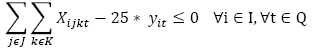
 (2)
(2)
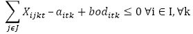
 (3)
(3)
 (4)
(4)
 (5)
(5)
 (6)
(6)
 (7)
(7)
 (8)
(8)
 (9)
(9)
 (10)
(10)
 (11)
(11)
 (12)
(12)
 (13)
(13)
 (14)
(14)
 (15)
(15)
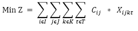
The objective function minimizes the total cost of transportation. To achieve this, the cost between each origin-destination pair and the number of loads to be transported between each farm and the industrial plant is considered (eq. 1).
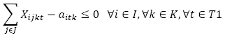
The total number of loads transported during the first period to each destination must be equal to or less than the number of available loads (eq. 2).
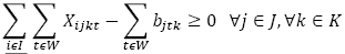
The total number of loads transported from each origin to each destination during the first four periods must be greater than or equal to the number of loads demanded of each product in each destination during the first four periods (eq. 3).
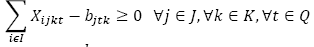
The total number of loads transported from each origin to each destination during the fifth period must be greater than or equal to the number of loads demanded of each product in each destination during the fifth period (eq. 4).
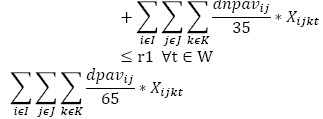
The total amount of transportation for each of the first four periods must be less than or equal to the total transportation capacity for each of the first four periods (eq. 5).
The total amount of transportation for the fifth period must be less than or equal to the total transportation capacity for each of the fifth period (eq. 6).
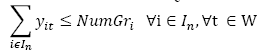
The number of cranes to be allocated to each subgroup of farms and in each of the first four periods must be less than or equal to the number of cranes available in each subgroup of farms for the first four periods (eq.7).
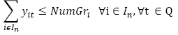
The number of cranes to be allocated to each subgroup of farms and in the fifth period must be less than or equal to the number of cranes available in each subgroup of farms for the fifth period (eq. 8).
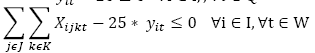
More than two cranes should not be allocated to the same farm for each of the first four periods (eq. 9).
More than twenty-two cranes should not be allocated to the same farm for the fifth period (eq. 10).
The maximum payload capacity that can be dispatched for each crane during the first four periods is 275 loads (eq. 11).
The maximum payload capacity that can be dispatched for each crane during the fifth period is 275 loads (eq. 12).
The total number of loads transported during the first period plus the warehouse of each farm and product for the first period must be less than or equal to the stock of logs per farm in the first period (eq. 13).
The volume of logs to be sent from each forest plus the quantity remaining in inventory for the subsequent period is equal to the quantity produced during the current period plus the quantity from the inventory of the previous period (eq. 14).
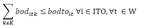
The warehouses of the subgroup of farms with harvests by means of logging towers must have an amount less than or equal to 80 in each of the first four periods (eq. 15).
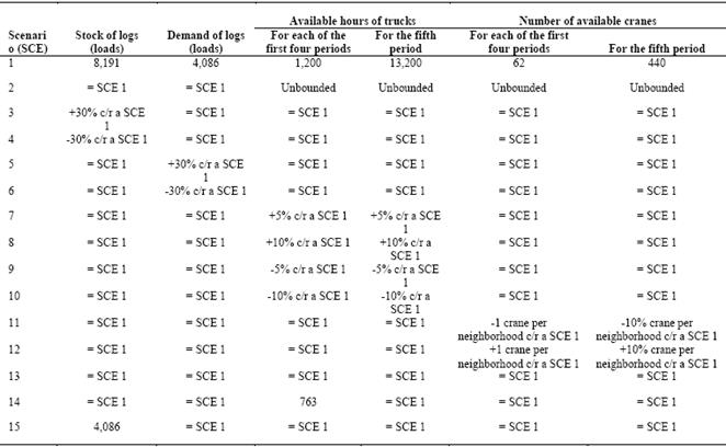
2.5. Test scenarios
The test scenarios used in the study are summarized in Table 1. All scenarios start from the baseline of scenario 1 and only one parameter is modified at a time to quantify the impact of this parameter on the result. SCE= 1 indicates that said parameter had the same value as in scenario 1.
Source: The authors.Table 1: Testscenarios used.
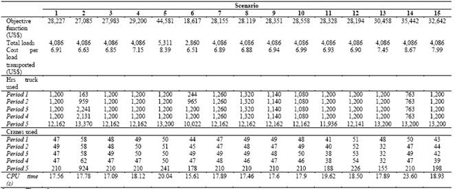
3. Results and discussion
Table 2 shows the results for the 15 proposed scenarios. Scenario 1 has a transportation cost of US$6.91 per load, uses 100% of the transportation capacity during the first four days and plans to use only 92% of the transportation capacity during the next 11 days. Alternately, the cranes achieve an average use of 77% during the first four days, and lowering the utilization of said cranes to 48% is planned for the next days of the period.
Scenario 2 achieves a cost (objective function) that is 4% lower with respect to the baseline scenario (scenario 1), but it must be taken into account that this scenario considers an unlimited capacity of transportation and payload, which generates the lowest cost of all scenarios with the same demand. The result in scenario 2 shows a marked trend to expect future periods to perform the transportation of logs because the forest farms that began to have stock permit found a better origin/destination combination, allowing for a reduction of the transportation costs. However, the need for transportation is completely unbalanced because it requires increasing the transportation capacity by more than five times in the period from 1 to 2 and more than double in the period from 2 to 3. This can be seen in column 2 of Table 2, regarding the number of hours of truck use. Regarding the cranes, the results show the same trend as for the case of transportation, but the differences are not so marked in each of the first periods; however, it indicates that more cranes are used than in the baseline scenario. This extreme flexibility in relation to the payload and transportation capacity is virtually impossible to achieve in reality. However, it is interesting to consider the possibility of counting on a degree of flexibility in the payload and transportation capacity to perform transportation programs with varying ability to delay or advance the transportation of logs and, thus, reduce costs.
Scenarios 3 and 4 consider variations in the stock of logs and achieve differences between -1% and 3% of the transportation costs in comparison to the baseline scenario, although it is expected that, by increasing the availability of loads by 30% in scenario 3, the cost of the freight decreases. Thus, it is important to take into account the order of magnitude in relation to the variation of the cost. Alternately, scenario 4 reduces the number of loads by 30% in comparison to the baseline scenario and generates a cost that is 3% higher than that of scenario 1.
Increasing the availability of payloads by 30% requires a significant increase in production, which requires extending the production shifts or hiring additional production lines. Any of the alternatives has an extra cost higher than US$0.06 per load (-1% in comparison to the baseline scenario), which is reduced from the transportation cost in comparison to the baseline scenario.
Scenarios 5 and 6, which vary in the demand of loads by +/- 30%, respectively, are relatively common for various reasons. Among these is the need to enter with more loads of logs because the industrial plants are processing a given type of log and the programmed amount of products for the next shipment has not been achieved. Then, the input of additional loads of logs to finish the production on time is urgently required. On the contrary, drops in the demand of loads despite not being so frequent can be presented as a result of unexpected failures in industrial plants, and the dispatch of loads must be stopped to repair the failure. Scenario 5 poses a hard restriction to the model because the demand of loads is increased by 30% with respect to the base scenario and the stock of logs and the capacity of loading and transportation are maintained. The higher quality logs present high demand and, generally, a low stock in farms without gaps between stock and demand, generating a critical scenario. The model allows finding a feasible solution that has an additional cost of 21% with respect to the baseline scenario. Transportation capacities are 100% utilized in both the first four days and the remaining 11 days. In the same line, this scenario requires activating the greatest number of cranes in all scenarios to load the trucks. An average of 81% of the cranes must be used during each of the first four days. The resolution time is also the highest of all scenarios, showing that the model is addressing a more complex situation than the other scenarios.
On the contrary, scenario 6, with a 30% increase in the demand of logs over the baseline scenario, has a 6% lower cost than the baseline scenario.
Scenarios 6, 7, 8, 9 and 10 consider modification to the transportation capacity with respect to the baseline scenarios. Scenarios 7 and 8 consider +5% and +10% of the transportation capacity with respect to scenario 1. The greater availability of transportation allows for finding an origin/destination combination that is 2 cents cheaper than that of the baseline scenarios. In the same line, scenario 8 continues to reduce the transportation costs by having greater transportation capacity, but it is still more marginal than the baseline scenario rather than scenario 8. Both scenarios show that the standard transportation capacity of the baseline scenario is virtually on the top of the economic optimum because although continuing to increase the transportation capacity allows for the reduction of costs, this reduction is marginal. This is corroborated by comparing the number of truck hours used in scenario 2, which had no limits in terms of the transportation capacity, i.e., in this scenario, the truck hours used are optimal for achieving the lowest possible transportation cost, and the truck hours used in scenarios 7 and 8 represent 92% and 96%, respectively, that of scenario 2 for the first 4 days and 91% for the remaining 11 days.
On the contrary, scenarios 9 and 10 consider -5% and -10%, respectively, the transportation capacity with respect to scenario 1. The lower transportation availability raises the transportation costs by approximately 1%, but again, the movements in the costs are quite marginal.
Of these four scenarios, it is possible to analyze that modifications of +/-10% in the amount of transportation for these scenarios that corresponds to +/- 240 truck hours per day generates no strong impacts on the transportation costs. This is due to the high flexibility of the model in terms of moving forward or delaying the delivery of the loads by at least 4 days. This accommodates the daily dispatch of loads according to the transportation capacity and thus meets at the fourth day with all customers at slightly higher or lower costs than those obtained with the standard transportation capacity.
Finally, scenarios 11 and 12 consider modifications to the number of available cranes per geographic area for truck loading. Scenario 11 considers one crane less per geographic area for each of the first four days than for the baseline scenario. The lower availability of cranes suggests the necessity of generating a set of origin/destination pairs different from those of the baseline scenario, as a product of the impossibility of loading in certain farms. Although the transportation cost of scenario 11 is higher than that of the baseline scenario, it is only 0.35 higher. The opposite effect but with an equal order of magnitude is observed in the results from scenario 12. The high availability of cranes considered by the baseline scenario and the possibility of moving forward or delaying the delivery of loads by up to four days allows for changes in the loading capacity to be absorbed by the system without strong impacts on the transportation costs.
In addition to the 2 above presented and solved scenarios, three additional scenarios that correspond to border scenarios for the first four periods of the model were considered.
As discussed in several contexts, the developed model allows for moving forward or delaying the delivery of the loads by up to 4 days maximum. This allows for freedom in the model to find the set of origin/destination combinations that minimizes the total transportation cost. To quantify the magnitude of the additional cost that assumes not having the freedom of moving forward or delaying the delivery of the loads, scenario 13 was run with the same parameters as scenario 1 or the baseline scenario and the model was modified to restrict it such that the loads demanded of each product in each destination should be delivered in the same period in which they were demanded.
The freight cost of scenario 13 or the scenario with fixed demand is where the advance or delay of the delivery of loads is 7.9 higher than that of the baseline scenario. This represents US$0.54 per load.
Scenario 14 has the same parameters as scenario 1 but 36% less transportation capacity for each of the first four periods, which reduced the truck availability per period from 1,200 hours to 763 hours. After performing successive approach runs, it was determined that scenario 1 cannot be solved with less than 763 truck hours for each of the first four periods. This decline in the transportation availability generates a rise in the average cost of transportation by 25% with respect to scenario 1. Although it is unlikely that the transportation availability is reduced by 36% due to fewer trucks as a product of mechanical failures, it is possible that this takes place as the result of a strike. The developed model allows for finding a feasible solution due to the flexibility of the load dispatch.
Finally, scenario 15 also poses a hard constraint to the model because, by considering the same parameters as for scenario 1 but maintaining both the supply and demand of each of the products, the offer is reduced to only the 4,086 demanded loads. The model continued to have the possibility of moving forward or delaying the delivery of loads by up to four days, but, at the end of the fourth period, all available loads should have been dispatched. This increases the transportation cost by 16% compared to that of scenario 1, resulting in US$1.08 more per load.
Source: The authors.Table 2: Results.
4. Conclusion
The problem described in this study is a real-world problem solved only by experience in the forestry company. The mathematical model constructed and detailed in this work solves all of the raised instances accurately, which permits its use as a valuable tool for the aid of decision-making against the problem of daily planning of both cranes and trucks for the dispatch of logs.
The model proposed allows for accurate solutions to different scenarios to be found by first knowing the feasibility of each one and their associated costs. Thus, to comply with the client’s expected deliveries, anticipating the problems is crucial. Changes in the demands or in the capacities of loading and transportation should be taken into account in making decisions regarding the evaluation of costs and deliveries to each customer, with an average computation time of 20 seconds.
The model developed without a fixed demand per period allows for balancing the use of the transportation capacity considering a later equitable programming of the transportation for all periods. That is, considering that different scenarios were established to incorporate the inherent variability of forest operations.
Acknowledgements
This study was partially supported by the grants: BasalConicyt-FB0816 and Ecos/Conicyt, Nº C13E04 and Mininco Forest Company.
References
Referencias
Rönnqvist, M., Optimization in forestry, Mathematical Programming, 97(1-2), pp. 267-284, 2003. DOI: 10.1007/s10107-003-0444-0
Chauhan, S.S., Frayret, J.M. and LeBel, L., Multi–commodity supply network planning in the forest supply chain, European Journal of Operational Research, 196(2), pp. 688-696, 2009. DOI: 10.1016/j.ejor.2008.03.024
Carlsson, D. and Rönnqvist, M., Supply chain management in forestry–case studies at Sodra Cell AB, European Journal of Operational Research, 163(3), pp. 589-616, 2005. DOI: 10.1016/j.ejor.2004.02.001
Olsson, L. and Lohmander, P., Optimal forest transportation with respect to road investments, Forest Policy and Economics, 7(3), pp. 369-379, 2005. DOI: 10.1016/j.forpol.2003.07.004
Troncoso, J., D´Amours, S., Flisberg, P., Rönnqvist, M. and Weintraub, A., A mixed integer programming model to evaluate integrating strategies in the forest value chain–A case study in the Chilean forest industry, CIRRELT working papers, 2011-28.
Linfati-Medina, R., Pradenas-Rojas, L. and Ferland J., Aggregate planning in forest harvest: A mathematical programming model and solution, Maderas-Cienc Tecnol 18(4), pp. 555-566, 2016, DOI: 10.4067/S0718-221X2016005000048.
Cómo citar
IEEE
ACM
ACS
APA
ABNT
Chicago
Harvard
MLA
Turabian
Vancouver
Descargar cita
CrossRef Cited-by
1. Ignacio Ortiz de Landazuri Suárez, María José Oliveros Colay. (2021). Design of Comminution Plants in the Ceramic Industry Using a Simulation-based Optimization Approach. Ingeniería e Investigación, 41(3), p.e87761. https://doi.org/10.15446/ing.investig.v41n3.87761.
Dimensions
PlumX
Visitas a la página del resumen del artículo
Descargas
Licencia
Derechos de autor 2017 DYNA

Esta obra está bajo una licencia internacional Creative Commons Atribución-NoComercial-SinDerivadas 4.0.
El autor o autores de un artículo aceptado para publicación en cualquiera de las revistas editadas por la facultad de Minas cederán la totalidad de los derechos patrimoniales a la Universidad Nacional de Colombia de manera gratuita, dentro de los cuáles se incluyen: el derecho a editar, publicar, reproducir y distribuir tanto en medios impresos como digitales, además de incluir en artículo en índices internacionales y/o bases de datos, de igual manera, se faculta a la editorial para utilizar las imágenes, tablas y/o cualquier material gráfico presentado en el artículo para el diseño de carátulas o posters de la misma revista.