DYNA

1. Introduction

Atmospheric convection, which leads to air mass circulation, is generally considered to result from the lower atmosphere acting as a heat engine, with the kinetic energy for convection deriving from differences in temperature, according to the general principle that hot air rises and cold air sinks. Makarieva et al. [3,4], in the Biotic Pump Theory (BPT), have argued that cloud-forming and the resulting condensation, fuelled by evapotranspiration from closed-canopy rainforest, removes water vapour molecules from the gas phase. That removal disturbs hydrostatic equilibrium and makes air circulate under the action of the evaporation/condensation force.

Evidence that surface airflow from the ocean to land is drawn in as a consequence of cloud condensation has come from a number of different sources. Poveda et al. [5,6] suggest that at 4° N over Colombia’s Chocó the high rate of evapotranspiration from the dense rainforest and the consequent cloud formation draws in humid surface winds from the Pacific Ocean.

Critics of the BPT argue that the movement of air which takes place during the condensation of water vapour is invariably an isotropic process, with the air moving from all directions simultaneously, thereby preventing any net, uni-directional flow [2]. The physical experiments, as undertaken and presented here, indicate instead that condensation can be anisotropic, thereby triggering a net, uni-directional flow.

2. Methodology

To test the underlying physics of the impact of condensation upon airflow, a dedicated structure forming a “square donut” was constructed. The experimental structure, Fig. 1, consists of two hollow columns, made of insulated PVC, 4.7 m high (internal), with an internal cross-sectional area of 1.38 m², connected at the top and bottom by ‘tunnels’ 2.35 m long.

Figure 1: This diagram shows the positioning of the sensors: Barometer (BAR), 2-D Ultrasonic Anemometer (UA) Thermocouple (T), and Relative Humidity Hygrometer, which also measures temperature (RH+T). The refrigeration coils, heating mat and rain-collector are also shown. It illustrates the set-up when the air circulation is clockwise, (gauze flaps). Sensors for RH+T have been placed at each of the three numerals at locations (1), (2) & (3), and BAR at locations (1) & (3). Location 1 is 0.05 m beneath the lower coil and 0.1 m below the junction of the upper tunnel with the right-hand column. Location 2 is 1.2 m above the floor of the right-hand column and location 3 is 0.5 m above the floor of the top tunnel. The top right T is 0.005 m from the upper cooling coil. The lower T in the right-hand column is 1.75 m up from the floor and the T in the left hand column is1.5 m from the floor. The T in the upper tunnel is 0.75 m from the junction with the right-hand column.

Source: Bunyard

Access to each column is by means of an insulated PVC door, with double glazing to allow a view inside. Two layers of copper refrigeration coils are located near the top of the right-hand column, around the four walls, connected to a 1 kW industrial refrigerator located some 3 m away on the floor of the laboratory. The cooling coils have a total surface area of 0.64 m² and take up one third of the cross-sectional area.

Calibrated sensors, including Class 1 thermocouples (T), Rotronic (accuracy ±0.8%) hygrometers (which also measure temperature) (RH+T), and barometric pressure gauges (PI642P accuracy ±0.062%) (BAR) provide measurements of changing conditions within the columns and tunnels every five seconds. A Novus logger transmits data from the four thermocouples and pressure gauges to the computer. The Gill 2-D ultrasonic Windsonic (accuracy ± 2%) anemometer (UA), measuring every second, is sited in various locations in the upper tunnel during the course of distinct experiments. One location for the anemometer is 0.1 m up from the floor of the upper tunnel and some 0.05 m from the junction between the tunnel and the right-hand column; another location is 0.5 m up from the upper tunnel floor and close to the junction of the tunnel with the left-hand column, therefore >2 m away from the cooling elements.

Lightweight gauze windflaps are located at the left end of the top tunnel and at each of the bottom tunnels. These flaps provide a visual indication of airflow direction when this is too low to be recorded by the anemometer.

The directionality of any airflow is either clockwise (down from the cooling coils and up the left-hand column), or counter-clockwise (up the right-hand column from the heating mat, past the cooling coils, and down the left-hand column). The Gill anemometer does not record directionality when airflow falls below 0.05 ms^-1, and does not record air speed below 0.01 ms^-1. Because of the way the anemometer is mounted, a rightwards or clockwise airflow is recorded as lying between 170° and 190°, and a leftwards or counter-clockwise flow as lying between 0°-10° and 350° -360°.

At the end of each experimental run, the frozen condensate on the cooling coils melts and the “rain” is gathered by means of a sloping-plane, hard plastic sheet, with a gutter at its lowest end.

3. Equations

Standard physics [7,8] are applied throughout to interpret the experimental results. The three variables of temperature, barometric pressure and relative humidity are used to calculate the partial pressure of water vapour (ppwv) using the exponential equation of Clausius-Clapeyron, [7] p.165. Eq. (1) & (2). Since at an atmospheric pressure of 1013.25 hPa, p 2 , water boils at 373 K, represented as 𝑇 2 , it is possible to substitute for 𝑝 2 and 𝑇 2 . The saturated partial pressure of water, 𝑝 1 .at each temperature, 𝑇 1 can be determined as follows:

Eq. (1) can be rewritten as:

In Eq. (1) & (2), Q, latent heat of evaporation is 40.65 kJ mol^-1, R, the ideal gas constant, is 8.31 J K^-1 mol^-1. The actual partial pressure of water vapour, 𝑝 1 , in the three numbered locations in Fig. 1, is given by multiplying the result by the relative humidity, RH, as measured by the hygrometers.

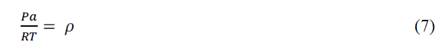
The air density is obtained through the use of the equation of state for ideal gases, [8 p.86]:

Where 𝑝 is the barometric pressure, hectopascals (hPa), 𝜌 is the air density in kgm^-3, 𝑅 is the ideal gas constant, J K⁻¹mol⁻¹ and 𝑇 is the temperature in Kelvin. Since 𝑅 varies with the degree of humidity, Eq. (4), is used with the values 287 J K^-1kg^-1 for dry air and 461 J K^-1kg^-1 for water vapour [8, p.89]:

To obtain q, the absolute humidity of water vapour kg per kg of moist air the following formula is used where 0.621 (18/29) is the ratio of the effective molecular weights of water vapour and dry air, [8, p.127]:

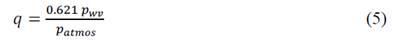
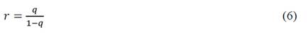
P _atmos is the barometric reading at that moment in time for the three locations and 𝑝 𝑤𝑣 is the partial pressure of water vapour, as calculated, at the same time of reading. When the value of q is applied to Eq. (4), it gives the value of R, the ideal gas constant for moist air, as water vapour is added or removed. 𝑟 is the absolute humidity of water vapour in dry air, hence kg of water vapour per kg of dry air. To obtain 𝑟, Eq. (6), the absolute humidity for moist air, q, first needs to be converted to the absolute humidity for dry air, r [8, p.127]:

To calculate the specific humidity, h (water vapour in grams per cubic metre of moist air), the values of 𝑞 and 𝜌 (the air density in kgm^-3) are required, as are the values for R, see Eq. (4) and T, as derived from the experimental data.

The air density, 𝜌, in kgm^-3 is obtained Eq. (7), using the ideal gas equation, see Eq. (3), where the barometric pressure is given in pascals (Pa):

The humidity, h, of moist air, in grams per cubic metre will be obtained, Eq. 8, from the proportion of humidity, q, in a given air density 𝜌, as from Eq. (7):

Eq. (9) (mass*acceleration) provides the kinetic energy values (Ws) for changes in the partial pressure of water vapour, (𝑃𝑎 (𝑡 , and that of change in air density per second, (𝜌 (𝑡 . The gravitational constant, g, is taken as 9.81 ms^-2.

Using Eq. (10), the kinetic energy required in circulating all the enclosed air (V) in the columns and connecting tunnels, some 19.5 m³, can be estimated from the average air density at the time of measurement and from the measured air velocity. For example, at an average air density, 𝜌, of 1.25 kg m^-3, and a volume V of 20 m³, the total mass of air would be 25 kg. With a velocity, v, of 0.2 ms^-1, the kinetic energy required would be 0.5 W s [2].

Transforming Eq. (10) into Eq. (11) provides the means to convert the kinetic energy (Ws) from the rate of change of air density and of partial pressure into average airflow velocity in the entire structure (mass of air approximately 25 kg):

As McIllveen [8, p.443] points out, thermo-dynamically, it is relatively straightforward to calculate the temperature increase in each kilogram of air as condensation takes place:

Where T is Kelvin; L is the latent heat of vaporisation of water vapour directly to ice, 2.9 MJ kg^-1; and 𝐶 𝑝 is the heat capacity of dry air at constant pressure, 1,000 J kg^-1K^-1.

McIllveen gives the example of 1 gram of water vapour condensing into liquid water and shows that it will warm 1 kg of air by 2.5 °C: a substantial amount.

The condensation of water vapour leaves the remaining air denser, which combined with its expansion into the partial vacuum from condensation causes the temperature to decline. The relationship between temperature change and air density change is as follows [8] p.444:

Where 𝑇 𝑣 is the virtual temperature of the water vapour; 𝑇 is the actual temperature of the air; and q is the specific humidity of moist air, kg water vapour per kg moist air. For the condensation of one gram of water vapour in 1 kg of air at 0 °C, the temperature reduction would be 0.17 °C.

4. The concept of air parcels

In this paper, the term “air parcel” is used to describe the volume of the layer of air influenced by the cooling elements as it passes over them (see Fig. 1B). As indicated below, parcel size is determined by the condensate collected as rain at the conclusion of each experiment.

In all the experiments, a vertical airflow (upwards or downwards) was observed within 30 seconds after the cooling elements were switched on and condensation began to take place. The question here is how to calculate the volume of air as it passes up or down through the cooling elements during one second? Given that the length of tubing forming the cooling elements is 17.03 m and the diameter of the coils is 0.012 m, the surface area of the cooling elements is 0.642 m². In order to derive the volume, that surface area must be multiplied by the effective extension of cooling. By knowing the total quantity of condensate gathered at the conclusion of each experiment, the average volume of air that passes over the cooling elements during each second can be calculated.

From Eq. (5) (7) & (8), the absolute humidity, q, (at 5s intervals) in kg/kg moist air can be calculated for the air at the cooling coils and for the air ‘next in line’, as can the air density, (, kgm^-3 of moist air, and finally the humidity, h, in gm^-3. By subtracting the humidity, h, of the air at the cooling coils from the humidity of the air next in line, the result will be gm^-3 of water vapour which will have condensed over the 5s interval between one measurement and the next. By aggregating the difference in h for each measurement over the entire experiment, the total loss of water vapour to condensation per second can be calculated as if the cooling volume were 1 cubic metre in size. That volume, 1 m ³ , will exceed by a factor, x, the actual volume size of the parcel block that is passing over the coils. Therefore, the total condensate, c, as measured from the precipitate, multiplied by x, will be equal to the aggregate of water vapour condensed, h _x (gm^-3), the factor, x, being the number of times the actual block size divides into 1 m³. Since the surface area of the coils is 0.642 m², the factor x will be 1/0.642 ef , where ef is the average effective layer, Eq. 14:

From the data, h _x (gm^-3) can be obtained (Eqs. (2)-(9), and knowing the actual quantity of condensate, c, Eq. (15) will give factor x:

The effective layer, ef, is found to lie between 0.04 m and 0.08 m for different experiments, the difference being a consequence of the airflow velocity. Depending on the experiment, the average parcel volume per second varies from 0.03 m³ to 0.06 m³ (Figs. 7, 8). As both Fig. 7, 8 show, the curve of the aggregated condensation of water vapour against time follows a near-straight line with an R ² of 0.97, thereby providing justification for Eq. (14)-(15).

5. Results

The widely-accepted assumption is that the movement of air in condensation of water vapour is invariably an isotropic process, with the air moving from all directions simultaneously, preventing any net, uni-directional flow. The experimental results indicate instead that condensation can be anisotropic, and can lead to net airflow. Isotropic condensation is inherently unstable, given the improbability of equivalent conditions existing in all planes surrounding the point of condensation.

In all experiments, once refrigeration was switched on, airflow became apparent within 30 seconds, through movement of the gauzes, around the entire 14 m internal length of the structure.

Figs. 2, 3 show a clockwise airflow, correlated with the periods of refrigeration and water vapour condensation.

Figure 2: 6 March 2015. The upper curve, (left-hand axis), with its peaks, shows airflow speed, and the line a 15-second moving average. The horizontal curve shows airflow direction. Five cycles of switching refrigeration on and off, with corresponding peaks in airflow of up to 0.09 ms-1. The airflow was clockwise, at around 180°.

Source: Bunyard

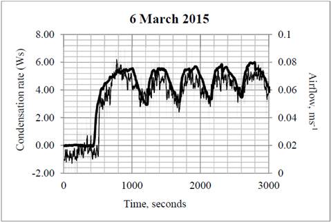
Figure 3: 6 March 2015. The upper curve shows the rate of change of the partial pressure of water vapour (ppwv) at the cooling coils, converted to Watt.seconds (left/hand axis). As before, the jagged curve shows airflow speed as a 10-second moving average. Because of low external temperatures, the compressor thermostat automatically switched the refrigeration on and off. The profile of the rate of decrease in ppwv shows peaks corresponding with peaks in the clockwise airflow ms-1.

Source: Bunyard

Fig. 4 shows a similar experiment, again with no internal heating. But on this occasion, the right column was observed to be 1 ºC warmer than the left, and the air had a slight counter-clockwise flow. When the cooling was switched on and off, in four cycles, the associated airflows were observed from the gauzes and anemometer to be counter-clockwise.

Figure 4: 19 April 2016. The upper graph and upper curve shows the rate of change of the partial pressure of water vapour (ppwv) at the cooling coils, converted to Watt seconds; the jagged curve shows airflow speed, as a 12-second moving average. Airflow was observed to be upwards over the cooling coils and therefore counter-clockwise. Airflow peaks were associated with the peaks of the partial pressure change (Ws). No artificial heating was applied, yet the tendency throughout was for the air in the right column to move upwards (approx. 0.02 ms-1). The lower curve shows the airflow and directionality, in this case counter-clockwise. The airflow peaks correlate with counter-clockwise directional flow (circa 10 and 350°).

Source: Bunyard

The periods of cooling in Fig. 4 correspond to the rise and fall in the rate of condensation. The times of cooling are on at 345 s, 1240 s, 2130 s, 3010 s and off at 630 s, 1530 s, 2440 s, 3490 s. At approx. 960 s, the airflow shows a short-lived peak of 0.07 ms^-1 which should be compared with the 0.12-0.14 ms^-1 longer-lived peak at 1510 s. A doubling of airflow circulation demands a four-fold increase in kinetic energy; 0.06125 W s compared to 0.245 W s.

Fig. 5, 6 both show the same experiment of 30 January 2016, with the cooling tubes switched on and off periodically, but with the heating mat on throughout. The flow of air was counter-clockwise (leftwards in the top tunnel). On account of directionality at the anemometer oscillating between around 1° or 360°, the graph shows a series of vertical lines.

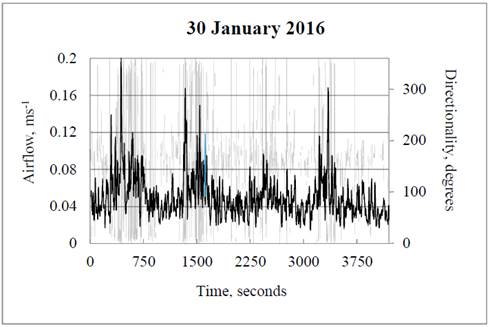
Figure 5: 30 January 2016. The black curve shows airflow speed as a 12-second moving average speed and the vertical, grey lines the direction of airflow. With the heating-mat on, four 5-minute cycles of refrigeration were carried out, with 10 minutes between each with the refrigeration switched off. Counter-clockwise airflow increased during the periods of cooling and subsided during the periods between. The directionality shows fluctuation between 10° and 350°.

Source: Bunyard

Figure 6: 30 January 2016 (same experiment as Fig. 5). The vertical, grey lines shows airflow speed, and the black curve a 12-second moving average. With the heating-mat switched on throughout, four cycles of refrigeration lasting 5 minutes each were carried out, with 10 minutes between each when the refrigeration was switched off. Counter-clockwise airflow increased during the periods of cooling and subsided during the periods between. The directionality as seen in Fig. 5 has been removed. However, the vertical lines of the airflow can be compared and matched with the directionality lines of Fig. 5.

Source: Bunyard

6. Experiments verifying air parcel concept

The air parcel concept, described in Methodology, enables the derivation of the rate of condensation, and the rate of an increase in air density as a result of the air becoming simultaneously more dense and cold. The calculation depends on a parcel of air with an average volume of between 0.03 m³s^-1 and 0.05 m³ s^-1, as calculated and contingent on the individual experiment; see Eq. (14) (15). Fig. 7, showing accumulated condensate, is obtained using the factor x to convert the aggregated total of h_x from 1 m³ down to the volume size of the parcel of air, namely 0.05 m³ s^-1. Experiments with airflow of 0.1 ms^-1 or less, (Fig. 7) tend towards the smaller parcel size of 0.03 m³ s^-1; experiments with airflow of 0.2 ms^-1 tend towards the higher virtual parcel size of 0.06 m³ s^-1, as shown in Fig. 8.

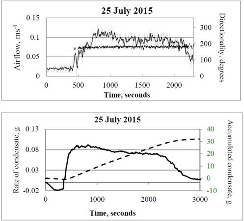
Figure 7: 25 July 2015. In the upper graph the upper curve shows airflow speed, as a 15-second moving average, and the horizontal curve shows airflow direction, in this experiment, clockwise. In the lower graph, the left-hand axis shows the dynamics of the rate of condensation in grams and the right-hand axis, with the dotted curve, shows its accumulation. Refrigeration was switched on at 350 seconds and off at 2250 seconds. The quantity collected and weighed from the rain trough was 32 g, which, when applied to give the average parcel size of the air undergoing refrigeration (0.06 m3) through using Eq. (14) (15) resulted in an accumulated condensation of 32 g (see Concept of Air Parcel). The slope of the accumulated condensate during the refrigeration has an R 2 of 0.97.

Source: Bunyard

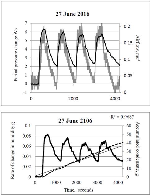
Figure 8: 27 June 2016. The upper graph shows the airflow over 4 refrigeration cycles (jagged black) and the partial pressure change in water vapour (upper curve, W s). The lower graph shows the change in humidity (peaked upper curve, g) and the aggregated accumulation of water vapour (dashed) through using Eq. (14) (15) and a volume size for the air parcel of 0.06 m3. The slope of the accumulated condensate during refrigeration has an R 2 of 0.97.

Source: Bunyard

7. Latent heat

The widespread scientific assumption is that the movement of air is isotropic, with cancellation of any net flow. The experiments indicate that condensation can be anisotropic, triggering a net, uni-directional flow. But the potential role of latent heat in air circulation nevertheless needs exploring. In the experiment shown in Fig. 9 of 30/01/2016, when the refrigeration was switched on, the air temperature at the cooling coils was immediately reduced, indicating that the latent heat released by water vapour condensation was wholly absorbed by the cooling tubes. Moreover, as refrigeration continued, with the temperature dropping so as to increase the rate of condensation, the associated increase in latent heat released per second did not show up as a levelling off of the temperature decline. Latent heat release thus cannot account for the upwards flow as shown in Fig. 4-6. Indeed, were it to be available for work, it would counter the downwards flow as in Fig. 2, 3, 7. The potential energy driving airflow in the condensation model must therefore come not from latent heat, but from partial pressure change. It is important to convert Eq. (13) to Ws through dividing by 𝐶 𝑝 , the heat capacity of dry air at constant pressure, namely 1,000 J kg^-1K^-1.

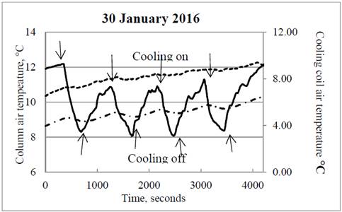
Figure 9: 30 January 2016 (same experiment as in Figs. 5, 6). The solid black curve shows temperature at the cooling coils, the dotted curve the temperature in the mid right-hand column below the cooling coils, and the punctuated curve the temperature in the lower left-hand column. The heating mat was on throughout four successive refrigeration cycles, with the on and off times shown by vertical arrows. The temperature decline on refrigeration indicates that the latent heat was annulled and could not be the cause of the enhanced upwards air circulation shown in Fig. 5, 6.

Source: Bunyard

Fig. 11 shows a significant correlation and regression (R² = 0.9074, p value <0.001) between airflow and the inverse pressure change from condensation. This is again consistent with the condensation model as an explanation of airflow. Finally, experiments with the anemometer placed more than 2 m away from the cooling coils and in the centre of cross-sectional area of the upper tunnel indicate that airflow is not limited to a thin stream but encompasses at least one third, if not all, the internal space of the structure. One experiment, Fig. 10, of 15 July 2016, is shown with clockwise circulation. The initial pre-refrigeration airflow is clockwise, amounting to approx. 0.05 ms^-1. Within 30 seconds of the refrigeration being switched on, the airflow, clockwise, has jumped to 0.16 ms^-1 and the rate of condensation from 0 to 7.8 W s.

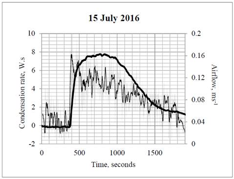
Figure 10: 15 July 2016. In this experiment showing clockwise flow, the anemometer is placed >2m away from the cooling elements. The initial sharp peak in airflow at 370 s (jagged curve) is matched by a sharp rise in the condensation rate of 7.7 W s (solid curve).

Source: Bunyard

Figure 11: 1 July 2014. In the upper graph the jagged grey curve shows airflow speed and the black solid curve the inverse rate of change in ppwv. The clockwise airflow (right axis) shows a close correspondence to the condensation rate (left axis). The lower graph shows the significant correlation (R 2 = 0.91, p value <0.001, Pearson’s Coefficient 0.92) between airflow and partial pressure change.

Source: Bunyard

8. Discussion

This paper is the result of more than 50 experiments, carried out between 2014 and 2017, held under different internal atmospheric conditions and analysed using conventional physics. The kinetic energy contributions from the partial pressure change in water vapour during condensation and from the air density change at the cooling coils are displayed in Table 1 for 50 different experiments. The cross-sectional area encompassed by each layer of the cooling coils is one third the cross-sectional area of the column. Therefore, the kinetic energy to move one third of the total volume of air contained in the structure is calculated on the basis of the anemometer reading. The direction of airflow, whether clockwise or counter-clockwise, is always consistent with anisotropic condensation. As Table 1 shows, the potential energy from partial pressure change is more than adequate to account for the kinetic energy of observed airflows, while the potential energy from cooling the same portion of air and accounting for density change, in general, falls short by a factor of 10 or more. Furthermore, the air density change per second shows no correspondence with the peak air velocity, thus indicating it cannot be responsible for the airflow, whether clockwise or anti-clockwise.

Table 1: KE characteristics of experimental data.

Source: Bunyard

In the experiment of 15/07/2016, with the anemometer more than 2 metres away from the cooling elements, significant airflow is detected throughout. Judiciously placed web-cams focussed on hanging gauzes, indicate that the change in the partial pressure of water vapour during the cooling cycles is sufficient to bring about convection throughout the entire structure, Fig. 10.

Neither air density changes nor latent heat release, whether the flow is clockwise or counter-clockwise, can explain the enhanced airflow as observed in all experiments undertaken [2]. Eq. (13) conforms to the kinetic energy required to account for the rate of change in the partial pressure of water vapour. That kinetic energy required by the air surrounding the locus of condensation is considerably more than that required to generate airflow around the structure (approx. 20 cubic metres of air), the assumption being that some is taken up in isotropic condensation and the remainder in anisotropic condensation, with sufficient power to overcome friction and turbulence. The positioning of the gauzes, with observation of their movement, and the anemometer, indicate that a convection cycle is generated.

Eq. (13) is critical in terms of explaining how the negative energy of partial pressure reduction transforms into a temperature change (negative) which, when multiplied by 𝐶 𝑝 , the heat capacity of dry air, some 1000 J K^-1 kg^-1, gives the Joules equivalent calculated for the change per second in the condensation rate (Pa converted into Ws).

Interpreting the experimental results in terms of the atmosphere at large requires caution, but they do suggest that they might apply where intense condensation occurs, especially in and above closed-canopy moist forest, in the tropics year-round and in temperate zones in summer. Eq. (13), being fundamental to the physics of ideal gases, will inevitably apply in the atmosphere at large as it clearly does in the experiments.

The conventional point of view is that the kinetic energy for convection derives from the general principle that hot air rises and cold air sinks. However, as Makarieva et al. [9] point out, when hot air rises in the lower atmosphere it cools because of expansion and when the same, but now cooler, air sinks it heats up, such that the overall gain or loss in kinetic energy is zero. The same cooling and heating happens when air expands and forces air elsewhere to compress; there is no net energy gain to do work. In other words, a strict application of the first law of thermodynamics to the atmosphere would yield a rate of kinetic energy generation equal to zero. In that respect, the buoyancy from latent heat release will be counteracted by cold air from above sinking, thus generating a hydrodynamic equilibrium.

According to the BPT [1] [3]), rainforests, year-round in the equatorial tropics and during the summer in boreal regions, feed the lower atmosphere with water vapour, up to 3 per cent of atmospheric pressure, and thereby provide the source material for cloud condensation. The depletion of water vapour and the resulting rarefaction of the local atmosphere in the locality of condensation cause convection over the forest, according to the BPT. From that point of view, it is the hydrological cycle, including water evaporation and condensation, which drives convection and therefore the circulation of the air masses. That is in sharp contrast to the orthodox view of convection and air mass circulation, which argues that the movement of the air mass drives the hydrological cycle through latitudinal differences in temperature, helped on by the buoyancy generated as a result of the release of latent heat [8 p. 444].

The proposition that a high rate of evapotranspiration from forested regions is a prime mover of major air mass convection remains contentious. Meesters et al. [10] rejected the BPT on the grounds that the ascending air motions induced by the evaporative/condensation force would rapidly restore hydrostatic equilibrium and thereby become extinguished. In reply Makarieva et al. [11] pointed out that condensation removed water vapour molecules from the gas phase and reduced the weight of the air column. That removal must disturb hydrostatic equilibrium and make air circulate under the action of the evaporation/condensation force.

In effect, the BPT states that the major physical cause of moisture fluxes is not the non-uniformity of atmospheric and surface heating, but that water vapour is invariably upward-directed as a result of the rarefaction of air from condensation [1].

Evidence in favour of the BPT has come from a number of different sources. Makarieva et al. [1] refer to data showing that precipitation over river basins which are covered in forest remains as high in the deep interior of the continent as at the coast, whereas river basins without forest show an exponential decline in rainfall as one passes from the coast inland. Spracklen et al. [12] have shown from their recent pan-tropical study of rainfall and land-cover, as indicated by the leaf area index (LAI), that satellite-derived rainfall measurements are positively correlated with the degree to which model-derived air trajectories have been exposed to forest cover.

Poveda et al. [5] [6] provide evidence that when the low level jet streams pass over forested regions precipitation levels stay high and constant, whereas over regions which lack forest, precipitation levels decline exponentially, just as the BPT suggests should happen. Poveda and his colleagues look at the low level Chocó jet and comment that the change in direction of the Pacific Austral Trade Winds from Easterlies to Westerlies just over the Equator at 4° N, may owe their abrupt switch to the unsurpassed degree of evapotranspiration and subsequent condensation over the Chocó in Colombia.

With more than 380,000 cubic metres per second of water vapour brought in from the Tropical Atlantic Ocean, the Amazon Basin functions on a far grander scale than the Chocó [13]. It would appear that evapotranspiration rates are sufficiently high over the rainforest to increase the volume of the Amazonian atmospheric river in the form of the South American Low Level Jet Stream as it approaches the western reaches of the Amazon Basin and is then deflected both upwards and southwards on encountering the Andes [14].

By focussing on temperature change rather than the pressure change when condensation occurs in the atmosphere, the latent heat release and subsequent air warming is deemed to more than compensate for the small reduction in temperature from the air expanding into the partial vacuum, Eq. (12) (13). However, the BPT takes into account the rarefaction of the atmosphere and the pressure change as water vapour condenses.

Moreover, in the experimental set-up latent heat release is eliminated by means of refrigeration and yet airflow against gravitational constraints is measurably enhanced as seen in Table 1 (AC) and from Fig. 4 & 5. That finding leaves partial pressure change from condensation as an important candidate for causing airflow and it raises fundamental questions concerning the supposed isotropy of airflow to the locus of condensing water vapour.

This paper describes an attempt to study the physics in a laboratory setting. The results have been significant and unambiguous. At the laboratory scale, using conventional physics such as is employed in climatological studies, the primary force driving convection appears to be the kinetic energy of imploding air as water vapour condenses, with a sudden reduction - >1200-fold - in the air volume of one gram-molecule of water vapour (18 g) as it transforms to liquid and ice. Hence, as air expands into the partial vacuum resulting from the condensation of water vapour it takes up heat from its surroundings which, together with the release of latent heat and the virtual warming of air, maintain the conservation of energy. Furthermore, because of physical differences above and below the refrigerated cooling coils, the process of eliminating the partial vacuum is anisotropic with the net result that condensation leads directly to uni-directional airflow.

9. Conclusions

The experiments described in this study, including those shown in Table 1, indicate that air density changes around the cooling coils are insufficient by more than an order of magnitude to bring about the observed airflows, and that more than sufficient potential energy, bound up in the partial pressure changes of condensation, is available to account for those same airflows. In the experimental set-up at least, both latent heat release and air density changes from the refrigeration can be ruled out as the cause of the consistent uni-directional net airflows. Anisotropic airflow to the locus of condensation remains the only candidate, in contrast to the accepted dogma that isotropic condensation is the norm and for which there is no evidence. In effect, the trigger for such directed airflows derives from distinct edge conditions in the vertical plane, above and below the area of condensation.

The laboratory demonstration of anisotropic condensation in causing enhanced air mass convection has implications for climate modelers who may have neglected this physical phenomenon in generating their climate algorithms. Many climate models may need revision. And it would strongly suggest that the great forests of the world play a fundamental role in air mass circulation through providing water vapour via evapotranspiration, and in bringing rain to the deep interior of continents [15] [16].

Acknowledgements

The experimental structure with its equipment and the actual experimentation made possible through the bounteous support of the Good Energies Foundation, Switzerland. Many thanks to Harry Fearnley for his careful scrutiny of the manuscript. Finally, we owe a profound debt to Jon Tinker for his help in the writing of the manuscript and his persistent questioning of the methodology and conclusions.

References

Referencias
Makarieva, A.M. and Gorshkov, V.G., Biotic pump of atmospheric moisture as driver of the hydrological cycle on land. Hydrology and Earth System Sciences, 11, pp. 1013-1033. DOI: 10.5194/hess-11, 2007.
Bunyard, P., Poveda, G., Hodnett, M., Peña, C. and Burgos, J., Experimental evidence of condensation-driven airflow. Hydrol. Earth Syst. Sci. Discuss., 12, pp. 10921-10974, 2015.
Makarieva, A.M., Gorshkov, V.G. and Li, B.L., The key physical parameters governing frictional dissipation in a precipitating atmosphere. Journal of the Atmospheric Sciences, 70, pp.2916-2929. doi:10.1175/JAS-D-12-0231.1, 2013.
Makarieva, A. M., Gorshkov, V. G., Sheil, D., Nobre, A. D., Bunyard, P. P., & Li, B.-L. Why does air passage over forest yield more rain? Examining the coupling between rainfall, pressure and atmospheric moisture content. Journal of Hydrometeorology, 15(1), pp. 411-426. doi:10.1175/JHM-D-12-0190.1, 2014.
Poveda, G. and Mesa, O.J., On the existence of Lloro (the rainiest locality on Earth): Enhanced ocean-land-atmosphere interaction by a low-level jet. Geophysical Research Letters, 27(11), pp. 1675-1678. DOI: 10.1029/1999GL006091, 2000.
Poveda, G.L., Seasonal precipitation patterns along pathways of South American low-level jets and aerial rivers. Water Resour. Res., 50, pp. 98-118. DOI: 10.1002/2013WR014087, 2014.
Daniels, F. and Williams, J.W., Physical Chemistry (International Edition). New York: John Wiley & Sons, 165 P, 1966.
Mcllveen, R., Fundamentals of Weather & Climate (2nd ed.). Oxford: Oxford University Press, 2010.
Makarieva, A.M., Gorshkov, V.G. and Li, B.L., Where do winds come from? A new theory on how water vapor condensation influences atmospheric pressure and dynamics. Atmospheric Chemistry and Physics, 13, pp. 1039-1056, 2013.
Meesters, A.G.C.A., Dolman, A.J. and Bruijnzeel, L.A., Comment on “Biotic pump of atmospheric moisture as driver of the hydrological cycle on land” by Makarieva, A.M. and Gorshkov, V.G., Hydrol. Earth Syst. Sci., 11, pp. 1013-1033, 2007. Hydrol.Earth Syst. Sci., 13, 1299-1305. Available at: http://www.hydrol-earth-syst-sci.net/13/1299/2009/. Doi: 10.5194/hess-13-1299-2009
Makarieva, A.M. and Gorshkov, V.G., Reply to A. G. C. A. Meesters et al.'s comment on "Biotic pump of atmospheric moisture as driver of the hydrological cycle on land". Hydrol. Earth Syst. Sci., 13, pp. 1307-1311, 2009. DOI: 10.5194/hess-13-1307-2009
Spracklen, D.V., Arnold, S.R. and Taylor, C.M., Observations of increased tropical rainfall preceded by air passage over forests. Nature, 489, pp. 282-285, 2012. DOI: 10.1038/Nature11390.
Salati, E., The forest and the hydrological cycle. In: Dickinson, R., Geophysiology of Amazonia, pp. 273-296. New York: W & Sons, 1987.
Marengo, J.A., On the hydrological cycle of the Amazon Basin: A historical review and current state-of-the-art. Revista Brasileira de Meteorologia, 21(3), pp. 1-19, 2006.
Bunyard, P.P., How the biotic pump links the hydrological cycle and the rainforest to climate: Is it for real? How can we prove it? (F.D. Publicaciones:, Ed.) Bogotá, Cundinamarca, Colombia: University of Sergio Arboleda, [online]. 2014. ISBN 978-958-8745-89-3. Available at: http://repository.usergioarboleda.edu.co/bitstream/handle/ 11232/397/How%20the%20biotic%20pump.pdf?sequence=2
Eiseltová, M., Pokorný, J., Hesslerová, P. and Ripl, W., Evapotranspiration – A driving force in landscape sustainability. Chapter 14, (A. Irmak, Ed.) InTech. DOI: 10.5772/19441, 2012.
Cómo citar
IEEE
ACM
ACS
APA
ABNT
Chicago
Harvard
MLA
Turabian
Vancouver
Descargar cita
CrossRef Cited-by
1. Peter Bunyard, Rob de Laet. (2024). Handbook of Climate Change Mitigation and Adaptation. , p.1. https://doi.org/10.1007/978-1-4614-6431-0_206-1.
2. Douglas Sheil. (2018). Forests, atmospheric water and an uncertain future: the new biology of the global water cycle. Forest Ecosystems, 5(1) https://doi.org/10.1186/s40663-018-0138-y.
3. Aleš Kučera, Pavel Samec, Aleš Bajer, Keith Ronald Skene, Tomáš Vichta, Valerie Vranová, Ram Swaroop Meena, Rahul Datta. (2021). Soil Moisture Importance. https://doi.org/10.5772/intechopen.93003.
4. Peter Paul Bunyard, Martin Hodnett, Carlos Peña, Javier D. Burgos-Salcedo. (2019). Further experimental evidence that condensation is a major cause of airflow. DYNA, 86(209), p.56. https://doi.org/10.15446/dyna.v86n209.73288.
5. Peter Bunyard, Rob de Laet. (2025). Handbook of Climate Change Mitigation and Adaptation. , p.1203. https://doi.org/10.1007/978-3-031-84483-6_206.
6. Peter P Bunyard, Eliza Collin, Rob de Laet, Martin Hodnett, Morel Fourman. (2024). Restoring the earth’s damaged temperature regulation is the fastest way out of the climate crisis. cooling the planet with plants. International Journal of Biosensors & Bioelectronics, 9(1), p.7. https://doi.org/10.15406/ijbsbe.2024.09.00237.
Dimensions
PlumX
Visitas a la página del resumen del artículo
Descargas
Licencia
Derechos de autor 2017 DYNA
Esta obra está bajo una licencia internacional Creative Commons Atribución-NoComercial-SinDerivadas 4.0.
El autor o autores de un artículo aceptado para publicación en cualquiera de las revistas editadas por la facultad de Minas cederán la totalidad de los derechos patrimoniales a la Universidad Nacional de Colombia de manera gratuita, dentro de los cuáles se incluyen: el derecho a editar, publicar, reproducir y distribuir tanto en medios impresos como digitales, además de incluir en artículo en índices internacionales y/o bases de datos, de igual manera, se faculta a la editorial para utilizar las imágenes, tablas y/o cualquier material gráfico presentado en el artículo para el diseño de carátulas o posters de la misma revista.