Publicado
Application of OpenFoam solver SettlingFoam to bedload sediment transport analysis
Aplicación del solucionador SettlingFoam de OpenFoam para el análisis del transporte de sedimento de carga de lecho
DOI:
https://doi.org/10.15446/dyna.v85n206.66804Palabras clave:
numerical model, sediment transport, mixture theory, turbulence model (en)modelo numérico, transporte de sedimento, teoría de mezclas, modelo de turbulencia (es)
Descargas
Recibido: 2 de agosto de 2017; Revisión recibida: 3 de mayo de 2018; Aceptado: 3 de junio de 2018
Abstract
Sediment transport is an important process for rivers and natural channels. The determination of sediment transport is a very complex process due to the high variability and changing nature of the factors that intervene. As a contribution to the description of this kind of phenomenon and to highlight the problems, the needs and potentials of the numerical approaches, OpenFOAM solver settlingFoam is used to simulate sediment transport in a rectangular channel. The model used constitutes a simplification of a complex procedure based on the application of a single parameter (alpha) to determine the fluid-sediment mixture features. High variability was found between the results from different alpha values. Nevertheless, there is a lack of information to determine the appropriate value of this parameter. However, even though the procedure applied and the results obtained have to be taken as a reference, this study provides valuable criteria for future research of this complex topic.
Keywords:
numerical model, sediment transport, mixture theory, turbulence model.Resumen
El transporte de sedimento es un proceso importante para ríos naturales, su determinación es un proceso complejo debido a la variabilidad y a la naturaleza cambiante de los factores que intervienen. Como una contribución a la descripción de este fenómeno y para enfatizar los problemas, las necesidades y las potencialidades de los enfoques numéricos, el solucionador settingFoam (OpenFoam) es utilizado para simular el transporte de sedimentos en un canal rectangular. El modelo utilizado constituye una simplificación de basada en la aplicación de un solo parámetro (alpha) para determinar las características de la mezcla fluido-sedimento. Alta variabilidad se reporta en los resultados para diferentes valores de alpha, sin embargo, existe poca información para determinar los valores apropiados para éste parámetro. A pesar de que el procedimiento aplicado y los resultados obtenidos deben ser tomados como referencia, este estudio provee criterios valiosos para la futura investigación de este tema tan complejo.
Palabras clave:
modelo numérico, transporte de sedimento, teoría de mezclas, modelo de turbulencia.1. INTRODUCTION
Sediment transport has considerable impact on river processes. It defines river morphology [1] and also has influence on water quality [2]. In North America the water pollution by sediments has an estimated cost of $16 billion per year [3]. Even though sediment transport of fine material 1.56 < d50(mm) < 28.6 has been studied in detail by [4 -7]. These studies don’t apply properly for coarser size sediments. Additionally, the slope plays an important role. The studies developed consider mainly mild slopes [8].
The study of sediment transport in steeper channels with coarse material is a complex process. Continuously changing driving forces, basin sediment production, and river bed conditions such as high gradients and large roughness elements result in high uncertainty in the quantification of sediment transport rates [1,9,10]. The uncertainty reported can reach some orders of magnitude [9,11]. Some equations have been proposed to account for bedload, movement thresholds, and channel roughness of steep channels with coarse material. Nevertheless, it tis concluded that there are more formulae than consistent data to verity them. Besides, no formula is proved to achieve consistent results, and no universal relation has been defines between bedload discharge and hydraulic conditions [12-14]. The essence, nature, and physics of sediment transport under these conditions (coarse material and steep channels) make its quantification a difficult process that still needs further investigation to achieve reliable results.
As an initial approach to achieve reliable tools to characterize sediment transport processes, in the present work, a sediment transport numerical model is applied to a study case. The case corresponds to a rectangular steel-glass channel with sediment entrance just at the inlet cross section. Thus, the settling features and transport velocity of a rectangular channel with water and sediment are determined. The main idea of developing the present application is to face the challenges, requirements, and potentialities (for a simple case) of this kind of models in order to project them to a simulation of more complex cases like natural rivers with steep slopes and coarse sediment.
2. METHODS
A numerical model that replicates the hydrodynamics of a two-phase (sediment and water) flow is developed to determine the distribution of the two phases along the domain, the sediment transport velocity, and the general flow variables pressure and velocity. The numerical analysis is performed with Open Filed Operation and Manipulation (OpenFOAM), an open source computational fluid dynamics (CFD) software package. It includes built-in applications, but can be used also to create new ones. The applications can be classified as solvers, used to find solutions to specific equations, and as utilities that can be seen as tools for data analysis and manipulation, generally results from the solvers (Open∇FOAM 2014). This software is used to solve the Navier-Stokes equations, the governing equations for this problem.
For modeling sediment transport OpenFOAM has a solver called settlingFoam. This model considers the mixture formed by water and sediment as a single phase instead of two separate phases. Considering each phase separately, a proper detail of the flow processes of each individual phase can be obtained. However, in the area where the two phases interact, there are difficulties in simulating the terms of the momentum transfer between the two phases.
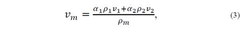
The main purpose of this solver is to determine the relative movement between the two phases. The density and pressure of the mixture are respectively defined with the following expressions:


The center velocity of the mixture volume is defined as follows.
The governing equations for the mixture flow, including the previous relations, are defined with the next expressions:
Mixture Continuity Equation,

Mixture Momentum Equation,

Drift Equation,

Where, αd represents the dispersed phase volume fraction. Pm , ρm , and um account for the average flow properties and vdj for the dispersion phase drift velocity. Finally, Γ is the diffusion coefficient composed by the molecular and turbulent viscosity.
Since the flow features of natural steep channels correspond to turbulent flow, the direct solution of the governing equations is not possible at a reasonable computational cost and simulation time. The resolution required by a DNS of isotropic turbulence that incorporates the viscous dissipation can be projected as four times the Kolmogorov length scale. Even for the smallest length scale the necessary mesh points is proportional to Re9/4. In open channel flow the resolution requirement is also dependent on the Reynolds number Re. It can be estimated as Nxyz = 2x10⁶(Re/300)2/7. Moreover, to solve the smallest eddies adequately the time step does not have to carry a fluid particle further than one cell [15]. Consequently, time step has to be decreased if cell size is decreased. Even for simple laminar cases, direct numerical simulations (DNS) have high costs [16]. A DNS is the most accurate, but even for low Reynolds number cases it has a high computational cost. It is impossible with the available tools to obtain a DNS for a complex geometry. Therefore, an alternative that balances accuracy and computational cost must be used [17].
2.1. Turbulence approach
To solve the Reynolds averaged Navier-Stokes equation, (RANS) two general categories can be applied. The first category, known as the eddy viscosity models, express the components of the Reynolds stress tensor as functions of the gradients of the mean velocity. These models can be classified in turn in isotropic (linear) or non-isotropic (non-linear), depending on which constitutive turbulence law they use. Additionally, depending on the procedure employed to determine the eddy viscosity, these models can be algebraic or differential. The second category depends on Second Moment Closure (SMC) models or Reynolds-Stress Transport (RST) models. For these types of models, the modelled solutions of RST equations are the components of the Reynolds stresses required to close the RANS [18].
2.2. Isotropic eddy viscosity models
The eddy-viscosity concept of Boussinesq is the base of most of the turbulence models. It assumes that the turbulence shear stresses are proportional to the main velocity gradient. Eddy-viscosity models express eddy viscosity vt as the product of a turbulence length scale, lt , and a turbulence velocity scale, ut .

As a function of the way in which these scales are calculated, the models can be divided in three kinds: zero-equation or algebraic eddy-viscosity models, one-equation models, and two-equation models.
2.3. Two-equation models
These models use one PDE (partial differential equation) for the length scale and one PDE for the velocity scale [18]. These models mostly use the same transport equation for the Turbulence Kinetic Energy (TKE) to calculate a local turbulence velocity scale  [15]. The most common two-equation models are the k-ε model and the k-ω models.
2.4. The k-ε model
This model utilizes an equation for the turbulent energy dissipation  , instead of the direct determination of the length scales, L, together with the kinetic energy k equation [17].
The semi-empirical k-equation and ε-equation are expressed as follows:
For the transport of the kinetic energy k:
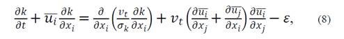
The terms in equation (8), from left to right, correspond to rate of change, convective transport, diffusive transport, production by shear, and dissipation.
For the transport of the dissipation rate ε:

The terms in equation (9), from left to right, correspond to rate of change, convective transport, diffusive transport, generation-destruction,

where, P is the generation term of the turbulent kinetic energy, and c1ε , c2ε , σε , cμ are empirical constants.
Turbulent eddy viscosity is then calculated when k and ε have been solved with the Prandtl-Kolmogorov expression [17].

2.5. Domain
The domain chosen for this study corresponds to a rectangular channel 30 cm wide by 45 cm high by 6 m long. As a prismatic small dimensions channel, the flow will be considered just in two dimensions (height and length). The two phases interaction simulated in settlingfoam are the fluid and sediment phase, established as the dispersed phase.
2.6. Boundary conditions
For the flow in a rectangular channel with the dimensions presented above, the boundary conditions include: two walls (upper and lower), inlet, and outlet. One velocity value was given for the inlet and walls. For the lower wall the non-slip condition (zero velocity) is set. The upper wall was given a slip condition. Outlet velocity is calculated. Furthermore, zero differential pressure is assigned to the outlet. For the walls and inlet, pressure is calculated.
Velocity and pressure were established based on laboratory conditions; k and ε were determined from the theory developed for turbulence models [19]. Here, the main relations used to determine the boundary conditions are presented.


where, u represents the main channel velocity, I is the turbulence intensity, Reo is the jet Reynolds number, L represents the length scale, and R is the hydraulic radius.
Three sediment volume fractions are simulated. There is not any guide to set the alpha ( αd ) volume as a function of the sediment conditions. Therefore, values of alpha corresponding to 1%, 0.1% and 0.01% of sediment are simulated to determine the effect of this parameter in the final solution.
2.7. Mesh
The domain is divided in uniform discrete cells of 0.01x0.01m, giving a total of 27,000 cells in the entire domain.
2.8. Schemes
The numerical method used by OpenFOAM is the finite volume method. For the time operator the Euller scheme is used. The Gauss linear scheme is used for the gradient and divergence operators. For the Laplacian operator, the Gauss linear corrected scheme is applied. Additionally, the interpolation scheme is set to linear. All of the schemes used have second-order accuracy [20]. Therefore, the simulations are considered second-order accurate. To verify solution’s convergence two parameters are analyzed. First, the residuals for the pressure, velocity and alpha equations are verified to drop to low values. The residuals are obtained from the absolute difference of the solution between the nth and (n-1)th . Additionally, change of the solution (alpha, velocity, and pressure) is tracked throughout the entire simulation to ratify that a steady-state solution has been achieved. All the simulations comprised 100,000 iterations. The final time corresponds to 2000s with a variable time step (between 0.01s).
3. RESULTS
As stated previously, some scenarios are considered to determine the influence of the parameter alpha and also to account for possible circumstances that may arise in the field. Summarizing, the simulations are performed with three different values of alpha: 0.01, 0.001, and 0.0001.
3.1. Residuals
The convergence criteria are verified with the residuals from the pressure, velocity and alpha equation. In Fig. 1 (a), (b) and (c) the residuals are presented for alpha = 0.01, 0.001, and 0.0001 respectively. As can be seen in the figures, the highest residuals correspond to pressure in all three cases. Comparing the different alpha values, the highest residuals correspond to alpha of 0.01.

Figure 1: Residuals of pressure, velocity, and alpha equations (a) αd = 0.01, (b) αd = 0.001, and (c) αd = 0.0001
Smaller residuals are obtained with small alpha values. This might indicate that small alpha values produce more stable solutions. For pressure, the residuals decrease two orders of magnitude when alpha decreases one order of magnitude. Similarly, residuals decrease two orders of magnitude when alpha decreases two orders of magnitude. For velocity, the residuals practically maintain their value for all alpha values simulated. A slight diminution is reported for the two smaller alpha values. However, considering the low value of velocity residuals this reduction is considered as non-significant. Alpha equations residuals are the lowest reported values. For the highest alpha value the residuals ranges from 10-8 to 10-10. For the two lower alpha values, residuals fall below 10-10. As observed alpha value adopted has considerable impact on the convergence of the solution.
3.2. Monitor point
The change in pressure, velocity, and alpha at a selected location (point: 3, 0.15) was monitored over the course of the simulation.
The results presented in Fig. 2 correspond to the parameters analyzed as follows. Fig. 2 (a) presents the alpha variation in the case of αd = 0.01. Fig. 2 (b) details pressure variation for αd = 0.001, Finally, Fig. 2 (c) shows the variation of the velocity for αd = 0.0001.

Figure 2: Change in the solution over time (a) alpha, αd = 0.01, (b) velocity, αd = 0.001, and (c) pressure, αd = 0.0001
Considering Fig. 2, the following can be reported. The pressure solution for αd =0.01 does not reach a constant value. However, the variation registered is small. This is in accordance with the small values reported for the residuals. In the case of alpha ( αd = 0.001), the constant values is reached around the time 1200s. For velocity and αd = 0.0001, the solution remains constant after the time 1500s. For all simulations (three alpha values), similar characteristics are obtained. In Fig. 2, a representative case of each parameter is presented.
3.3. Alpha
The alpha variation around the whole domain is presented in Fig. 3 for all three values of alpha considered. As can be seen in the figure, the data scale for (a) and (b) are the same. For (c) the scale is reduced to adjust the figure to the values of that case. Due to the high value of alpha in (a) the dispersed phase (sediment phase) is filling almost the entire domain. Being as the inflow of sediment is permanent during the simulation and the high sediment concentration, in this case the sediment phase occupies a high percentage of the channel.
In Fig. 3 (b), ( αd = 0.001) it can be seen that sediment has settled almost entirely approximately the 75% of the domain. The first quarter of the domain contains a higher amount of sediment. Nevertheless, this amount is smaller than the one settled in the channel bottom. For Fig. 3 (c) the reported results are similar to those obtained in Fig. 3 (b); the only difference is the absolute value of alpha.

Figure 3: Variation of alpha in the domain (a) αd = 0.01, (b) αd = 0.001, and (c) αd = 0.0001
3.4. Drift velocity
As can be observed in Fig. 4 (a), (b), and (c), the drift velocity shows exact correspondence to the alpha values. High velocity values correspond to small alpha values and small velocities match with high alpha values. Namely, the sediment phase will be dragged by smaller velocities than the fluid phase.

Figure 4: Variation of drift velocity in the domain (a) αd = 0.01, (b) αd = 0.001, and (c) αd = 0.0001
3.5. Velocity and velocity vectors
As presented in Fig. 5 (a) , (b), and (c), flow velocity presents a different pattern for αd = 0.001. For high and low alpha the flow configuration is similar. The flow domain, for intermediate alpha, presents recirculation zones following the pattern defined for alpha changes replicating what it is observed with drift velocity.

Figure 5: Variation of flow velocity in the domain (a) αd = 0.01, (b) αd = 0.001, and (c) αd = 0.0001
3.6. Vertical velocity profile
Vertical velocity profiles were obtained at the middle of the domain. The results are presented in Fig. 6. As can be observed, different velocity profiles were obtained with the different alpha values. The maximum flow velocity is reported for αd = 0.001 with a value of 0.044 m/s. The dissimilar behavior observed in the previous figures is also registered for the velocity profiles for each value of alpha. For αd = 0.01, a severe increase in the velocity is presented in the top of the domain. This can be caused for the change between sediment phase and boundary condition in a small distance (one cell).

Figure 6: Vertical velocity profiles
4. CONCLUSIONS
A numerical model was set to analyze sediment transport processes in a rectangular channel. The numerical model is based on mixtures theory. It constitutes a simple approach to a very complex problem. Well tested and strictly proven procedures like the discrete numerical solution of the Navier-Stokes equations and turbulence models were used in the present simulations. However, a simple method, that just considers a single parameter (alpha) to characterize the mixture, is applied to intend to replicate the natural process. As can be seen in the results, a considerable variability is found with the variation of alpha. Parameters such as flow and drift velocity report a dependence on the alpha value. Specifically, as alpha decreases the channel transport capacity appears to increase (drift velocity increases). Flow velocity presents a different behavior for the medium alpha used. With slight differences, the highest and lowest alphas show similar trends. Additionally, as has been pointed alpha has influence even in the stability and convergence of the equation’s solution. Conversely, no hint is available for the correct determination of this parameter. To obtain accurate results, a calibration and validation of the final alpha value must be performed. Thereby, a methodology can be stablished to define the correct alpha value.
This work and the application of settlingFoam can be considered as a first simple approach to the numerical simulation of sediment transport processes. The methodology applied here can be taken as the very first step to achieve a more realistic simulation. The simplicity found in the procedure can lead to the reduction in applicability of the method just for simple cases and the results as a reference of the real values. To set a more realistic numerical model an extensive investigation must be accomplished for both field conditions and model-required parameters.
REFERENCES
Referencias
López, R., Vericat, D. and Batalla, R.J., Evaluation of bed load transport formulae in a large regulated gravel bed river: the lower Ebro (NE Iberian Peninsula), J. Hydrol., 510, pp. 164-181, 2014.
Julien, P.Y., Erosion and sedimentation, 2nd ed. Cambridge; New York: Cambridge University Press, 2010.
Pons, L., Helping states slow sediment movement: a high-tech approach to clean water act sediment requirements, Agricultural Research Magazine, 51(12), pp. 12-14, 2003.
DuBoys, M.P., Etudes du regime du Rhone et de l’action exercee par les eaux sur un lit a fond de graviers indefiniment affouillable, Ann. Ponts Chaussees, 18, pp. 141-195, 1879.
Einstein, H.A., Formulas for the transportation of bed load, Trans ASCE, 107, pp. 561-573, 1942.
Meyer-Peter, E. and Müller, R., Formulas for bed-load transport, Proc 2nd Meet. IAHR Stockh., pp. 39-64, 1948.
Shields, Applicatioin of similarity principles and turbulence research to bed-load movement, California Institute of Technology, Pasadena, CA, 1936.
Lamb, M.P., Dietrich, W.E. and Venditti, J.G., Is the critical Shields stress for incipient sediment motion dependent on channel-bed slope?, J. Geophys. Res., 113(F2), May, 2008.
Carling, P.A. and Reader, N.A. Structure, composition and bulk properties of upland stream gravels, Earth Surf. Process. Landf., 7(4), pp. 349-365, Jul. 1982.
Papanicolaou, N., Bdour, A. and Wicklein, E., One-dimensional hydrodynamic/sediment transport model applicable to steep mountain streams, J. Hydraul. Res., 42(4), pp. 357-375, Jan. 2004.
Bathurst, J.C., Effect of coarse surface layer on bed-load transport, J. Hydraul. Eng., 133(11), pp. 1192-1205, Nov. 2007.
Gomez B. and Church, M., An assessment of bed load sediment transport formulae for gravel bed rivers, Water Resour. Res., 25(6), pp. 1161-1186, Jun. 1989.
Habersack H.M. and Laronne, J.B., Evaluation and improvement of bed load discharge formulas based on Helley-Smith sampling in an Alpine Gravel Bed River, J. Hydraul. Eng., 128(5), pp. 484-499, May 2002.
Martin, Y., Evaluation of bed load transport formulae using field evidence from the Vedder River, British Columbia, Geomorphology, 53(1-2), pp. 75-95, Jul. 2003.
Wilcox, D.C., Turbulence modeling for CFD, 3rd ed. La Cãnada, Calif: DCW Industries, 2006.
Reynolds, W.C., The potential and limitations of direct and large eddy simulations, in whither turbulence?, Lumley, J.L., Ed. Turbulence at the Crossroads, Springer, Berlin, Heidelberg, 1990, pp. 313-343.
Sturm, T.W. Open channel hydraulics, 2nd ed. Dubuque, IA: McGraw-Hill, 2010.
Bates, P.D., Lane, S.N. and Ferguson, R.I., Eds., Computational fluid dynamics: applications in environmental hydraulics. Hoboken, NJ: J. Wiley, 2005.
Menter, F.R. Two-equation eddy-viscosity turbulence models for engineering applications, AIAA J., 32(8), pp. 1598-1605, Aug. 1994.
Open∇FOAM, Open∇FOAM. The open source CFD toolbox, user guide, 2014.
Cómo citar
IEEE
ACM
ACS
APA
ABNT
Chicago
Harvard
MLA
Turabian
Vancouver
Descargar cita
Licencia
Derechos de autor 2018 DYNA

Esta obra está bajo una licencia internacional Creative Commons Atribución-NoComercial-SinDerivadas 4.0.
El autor o autores de un artículo aceptado para publicación en cualquiera de las revistas editadas por la facultad de Minas cederán la totalidad de los derechos patrimoniales a la Universidad Nacional de Colombia de manera gratuita, dentro de los cuáles se incluyen: el derecho a editar, publicar, reproducir y distribuir tanto en medios impresos como digitales, además de incluir en artículo en índices internacionales y/o bases de datos, de igual manera, se faculta a la editorial para utilizar las imágenes, tablas y/o cualquier material gráfico presentado en el artículo para el diseño de carátulas o posters de la misma revista.