Industrialization and growth: threshold effects of technological integration.

Los países disfrutan de las ventajas de industrialización en el crecimiento económico después de superar un cierto umbral de integración tecnológica en manufacturas. Algunos datos disponibles no rechazan esta hipótesis. Este rasgo del desarrollo es consecuente con las brechas observadas en tasas de crecimiento de largo plazo entre economías ricas y pobres.

Carlos Humberto Ortiz *

Javier Andrés Castro**

Erika Raquel Badillo***

*PhD. in Economics, Professor in the Department of Economics at Universidad del Valle and member of the research group on Growth and Economic Development (Cali, Colombia). E-mail: ortizc@univalle.edu.co. Address: A.A. 25360 (Cali, Colombia).

**Master Science in Economics, Professor and Director in the Department of Economics at Universidad del Valle and member of the research group on Growth and Economic Development (Cali, Colombia). E-mail: jacastro@univalle.edu.co. Address: A.A. 25360 (Cali, Colombia).

***Master(c) in Economics, member of the research group on Growth and Economic Development (Cali, Colombia). E-mail: erikabad@univalle.edu.co. Address: Calle 3B N° 96-19 Apto 601A, Barrio Meléndez, Cali (Colombia).

The authors thank Douglas Laing and José Ignacio Uribe for academic advice. Financial support from Universidad del Valle is gratefully acknowledged.

This article was received on January 2, 2009 and his publication approved on August 23, 2009

---

Resumen

Los países disfrutan de las ventajas de industrialización en el crecimiento econímico después de superar un cierto umbral de integración tecnológica en manufacturas. Algunos datos disponibles no rechazan esta hipótesis. Este rasgo del desarrollo es consecuente con las brechas observadas en tasas de crecimiento de largo plazo entre economías ricas y pobres.

Palabras clave: umbral de integración tecnológica, industrialización, crecimiento divergente, educación. JEL: F43, L16, L60, O11, O14.

Abstract

Countries enjoy the benefits of industrialization for economic growth after surpassing a certain threshold of technological integration in manufacturing. Some available data do not reject this hypothesis. This feature of development is consistent with the observed gaps in long-run growth rates between rich and poor economies.

Key words: threshold of technological integration, industrialization, growth divergence, education. JEL: F43, L16, L60, O11, O14.

Résumé

Les pays jouissent des avantages de l´industrialisation dans la croissance économique après avoir surpassé un certain seuil d´intégration technologique des manufactures. Les quelques données disponibles ne repoussent pas cette hypothèse. Ce trait du développement est conséquent avec les brèches observées dans les taux de croissance de long terme entre les économies riches et les pauvres.

Mot clés : seuil d´intégration technologique, industrialisation, croissance divergente, éducation. JEL : F43, L16, L60, O11, O14.

---

In spite of all the discussion on economic convergence, cross-country analyses of long-run economic growth reveal a divergent pattern. According to Madisson´s (1994) analysis over a sample of 21 countries, the ratio of the highest GDP per capita to the lowest increased from 3 to 17 between 1820 and 1989. And Pritchett (1997) estimates that from 1870 to 1990 the ratio of per capita income between the richest and the poorest countries increased by a factor of five.

This divergent pattern is also observed for more recent periods. Hall and Jones (1997) found that the ratio of GDP per worker of the richest one-fifth of countries to that of the poorest one-fifth of countries increased from 26 to 29 between 1960 and 1988. Easterly and Levine (2001) reported that divergence of per capita income has increased from 1960 to 1992. Their estimations in Table 1 show that the two higher fifths of countries grew faster than middle income countries, and these in turn grew faster than the two lower fifths.

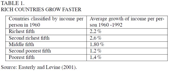
Hence, the world division among these three “clubs” –rich countries, middle income countries and poor countries- is deepening. A recent World Bank research report has confirmed this feature. Perry et al. (2006) showed that the unimodal distribution of per capita real income across countries in 1960 has become a trimodal distribution in 1999. They showed as well that since 1960 there has been convergence within these “clubs” but divergence amongst them. It is thus unavoidable to conclude that the income gap between rich countries and the remainder has been widening over a long period.

The existence of persisting growth gaps across countries was discovered by Kaldor. In his classic paper on the patterns of development he wrote: “there are appreciable differences in the rate of growth of labour productivity and of total output in different societies” (Kaldor, 1961, 179). This was the sixth pattern; the first five were as follows:

1. Output per worker shows continuing growth, with “no recorded tendency for a falling rate of growth of productivity”.

2. Capital per worker shows continuing growth.

3. The rate of return on capital is steady.

4. The capital-output ratio is steady over long periods.

5. Labour and capital receive constant shares of total income.

Kaldor´s patterns of development imply a world economic structure where convergence is not guaranteed. Historical experience of economic development supports this vision; even though a few previously underdeveloped economies have been able to take off, most underdeveloped economies have been unable to follow suit. Given this scenario, gaining an understanding of the underlying mechanisms of economic divergence is one of the most challenging tasks facing development analysts.

INDUSTRIALIZATIONAND ECONOMIC GROWTH

It was also Kaldor who put forward the thesis that cross-country variations of economic performance were related to industrialization:

Fast rates of growth are almost invariably associated with the fast rate of growth of the secondary sector, mainly manufacturing, and... this is an attribute of an intermediate stage of development (Kaldor, 1966, 7).

Following this line of research, Chenery, Robinson and Syrquin (1986) analyzed the relationship between industrialization and economic growth. Using data from a selected group of industrial and semi-industrial countries, and after identifying some unlikely exceptions –poverty traps, persistence of the Dutch disease phenomenon in the primary sector, and early development on export services, Chenery et al. claimed to have found enough evidence to support Kaldor´s hypothesis:

Is industrialization necessary to continued growth? Our models of the transformation suggest that the answer is generally yes. (...) We conclude that –on both empirical and theoretical grounds– a period in which the share of manufacturing rises substantially is a virtually universal feature of the structural transformation (Chenery et al., 1986, 350).

Murphy, Shleifer and Vishny also concurred to this viewpoint:

Virtually every country that experienced rapid growth of productivity and living standards over the last 200 years has done so by industrializing. Countries that have successfully industrialized –turned to production of manufactures taking advantage of scale economies– are the ones that grew rich, be they 18th-century Britain or 20th-century Korea and Japan (Murphy, Shleifer and Vishny, 1989, 1003).

Some twentieth-century experiences of economic development are consistent with this pattern. Newly industrialized countries are among the highest growing economies over the period 1965-1990; they are, in order of performance, Singapore (1), Korea (2), Taiwan (5), Hong-Kong (6), China (7), Indonesia (8), Japan (10), Malaysia (11), Thailand (18), Brazil (19) and Yugoslavia (20). On the other hand, all the lowest growing economies in the same period are non-industrialized countries (see Barro and Sala-i-Martin, 1995, Tables 12.1 and 12.2). Besides, the most recent successful experiences of economic take offs, China and India, are also related to industrialization and economic diversification.

Thus, industrialization matters. That is why the advice of Leontief for developing countries was the following:

Given the country mix of resources and the available technologies, the essence of the process of development [is] to create an economic system as similar as possible to the system of the most developed economies (Leontief, 1963, 164).

Hence, if industrialization is the key to economic development, why do we observe so very few cases of successful economic take offs? Why cannot we the underdeveloped countries catch the train of progress? This paper attempts to provide an answer. According to a certain vision of economic development, a period of structural transformation is previously required in order to take advantage of the external effects of industrialization on productivity, competitiveness and economic growth. During that period, national institutions and economic agents have to commit themselves to industrialize (Hirschman, 1958; Amsden, 1989; Landes, 1998). Coordination problems related to this commitment are perhaps what make it so difficult to gain access to the exclusive “club” of developed economies (Hirschman, 1958; Murphy, Shleifer and Vishny, 1989). In summary, our main hypothesis is that the causal relationship from industrialization to economic growth is non-linear: each society should endeavour to achieve some minimum level of manufacturing technological integration before it can reap the benefits of industrialization in economic growth.

In this structuralist vision, each country is considered as some kind of living being that ought to transform itself into an adult before being able to survive and compete successfully in the world markets. The latter analogy is based on empirical analyses of economic development. Chenery, Robinson and Syrquin (1986) identified that along the process of industrialization some structural changes take place –economies grow up. The main features of this structural transformation are, according to these authors, the following: changes in final demands, changes in intermediate demands and changes in international trade. The first structural change is the well-known Engel´s law: income elasticity of food demand is lower than 1; thus, the agricultural sector expands slower than the economy as a whole. The second structural change is what these authors refer to as input-output deepening:

As countries industrialize, their productive structures become more “roundabout” in the sense that a higher proportion of output is sold to other producers rather than to final users. (...), this phenomenon can be broke down into two parts: first, a shift in output mix toward manufacturing and other sectors that use more intermediate inputs; and second, technological changes within a sector that lead to a greater use of intermediate inputs (Chenery, Robinson and Syrquin, 1986, 57).

The third structural change is related to the evolution of international trade: comparative advantages change from the primary sector to the manufacturing sector. The following quotation is illustrative:

Through import substitution and the expansion of manufactured exports, developing countries shift away from the specialization in primary products that is characteristic of early stages of development. Underlying this shift are changes in supply conditions –accumulation of skills and physical capital plus the greater availability of intermediate inputs– as well as economies of scale based on a growing domestic market for manufactured goods (Chenery, Robinson and Syrquin, 1986, 63).

Hence, according to the structuralist vision of economic development, it might be true that only when a country´s structural transformation is sufficiently advanced it might open to world markets, become an exporter of manufactured goods and enjoy the benefits of industrialization –including higher growth rates.

Theoretical analyses that are consistent with this vision include growth and international trade models where learning-by-doing is the growth engine, such as those of Lucas (1988), Young (1991), Matsuyama (1992) and Ortiz (2004, 2008). In these models, and under an open economy regime, a country´s pattern of specialization is determined by its inherited advantages. Thus, advantages in high-learning economic activities, typically manufacturing, drive the economy along a superior path of economic development; whilst advantages in low-learning technological activities might lock the economy up in those activities and lead to sluggish economic growth.

Several reasons can be put forward in order to explain the strong economic externalities from the manufacturing sector. First, product diversification, and its important effects on productivity (Romer 1987, 1990), takes place typically in the manufacturing sector. Second, the continuous displacement of the technological frontier in the manufacturing sector allows the sector´s learning potential to remain high (Lucas, 1988; Young, 1993). Third, the manufacturing sector is characterized by intensive application of science and technology to transform intermediate goods and raw materials; moreover, the sector´s generation of new goods and new technologies induces the appropriation and diffusion of humanity´s most important productive force: scientific knowledge (Romer, 1986). Fourth, the productivity of the manufacturing sector, as producer of intermediate and capital goods, impinges directly on the system´s profitability (Sraffa, 1960) and the rate of economic growth (Rebelo, 1991). Fifth, the manufacturing sector typically enjoys internal and external economies that enhance aggregate productivity (Caballero and Lyons, 1990).

Some words of caution are required at this point. It is convenient to emphasize that there is nothing magical about manufacturing; other economic activities requiring an intensive use of intelligence and technology – informatics, communications, biotechnology, scientific research, etc.– may also become leaders of economic growth (Landes, 1998; Rodrik, 2007).

SOME EMPIRICAL SUPPORT

A Small Panel Data

According to the analysis of structural transformation (Chenery et al., 1986), economic diversification is directly related to production “roundaboutness”. It is thus convenient to test the diversification effects on economic growth by using a measure of interindustrial dependence as a proxy. In order to do that, a small panel data set containing such a measure is used in this analysis.

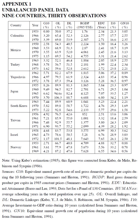
Based on Kubo´s work on cross-country comparisons of interindustrial linkages (Kubo, 1985), Kubo, de Melo, Robinson and Syrquin (1986) calculated comparable indices of aggregate interindustrial linkages using information from 30 input-output matrices of nine industrialized or semiindustrialized countries: Colombia, Mexico, Turkey, Yugoslavia, Japan, South Korea, Taiwan, Israel and Norway. Observations were taken for some years between 1950 and 1975. According to the authors, each country represented a different stage of structural change. To that extent, the sample may be thought of as being representative of the experience of economic development.

The procedure to calculate the mentioned indices was the following. First, the authors rearranged each matrix into 14 comparable economic sectors and calculated the matrix of technical coefficients A = [a_ij ], where a_ij is the technical coefficient measuring the amount (in value terms) of input i which is consumed in the production process of one unit of good j. Subsequently, they calculated the Leontief matrix, L = I - A, where I denotes the identity matrix of the same order as matrix A. Finally they obtained an index of overall linkages as follows: (OL) = f´(L´)^-1i, where OL is a scalar, f is a 14x1 weight vector whose elements add up to 1, i is a 14x1 unit vector, the apostrophe (´) denotes matrix transposition, and the power-1 denotes matrix inversion.

Let us decompose this expression: (L´)^-1i is a 14x1 vector whose elements measure the degree of backward technological integration of the corresponding sectors, i.e. each element measures the proportion of gross output which is produced in the economy per unit value of final demand in the corresponding sector. The final expression (OL) is then a weighted average of these measures, where the weights are taken from the representative structure of the final demand vector for a semi-industrial country (see Chenery, Robinson and Syrquin, 1986). These authors also obtain an index of domestic linkages (DL) by excluding imported intermediate inputs from the input-output matrix; the calculation is completely analogous to the previous one.

Appendix 1 exhibits the data on measures of interindustrial linkages, overall linkages (OL) and domestic linkages (DL), for the above panel of countries. It also includes the equivalent annual growth rates of per capita GDP during 10 years (G10), the real per capita GDP (RGDP), the average schooling years in the total population over age 25 (EDU), the average investment ratio in the next decade (I10), and the equivalent annual growth rate of population in the next decade (GN10).

Growth Regressions from the Panel Data

Appendix 1 is a small unbalanced panel. Using this information the growth regressions shown in Table 2 are run. x to heteroscedasticity –this hypothesis cannot be rejected at the 1 percent level– OLS estimates are corrected using White´s consistent covariance matrix. The dependent variable is the average annual growth rate of GDP for the next 10 years (G10).

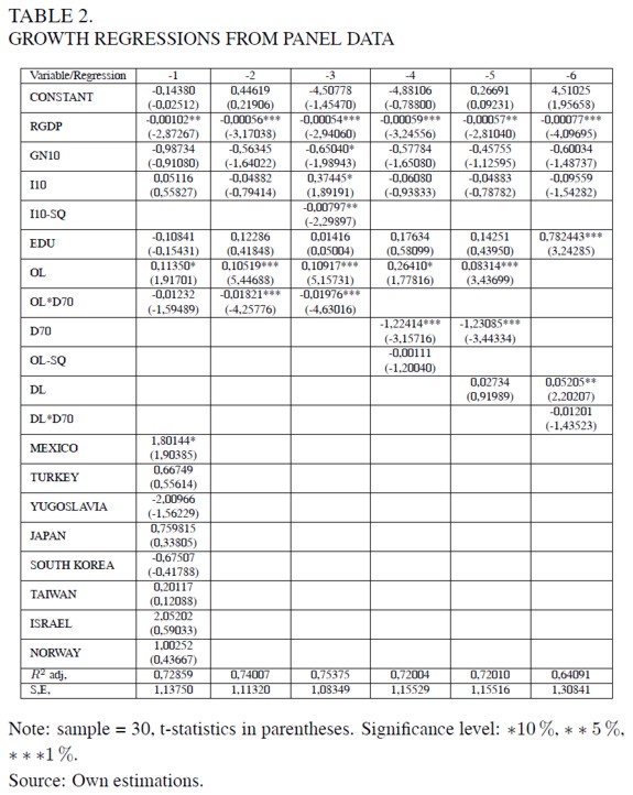
The first set of included independent variables (the basic set from now on), are the real per capita GDP (RGDP), the average annual growth rate of population in the following decade (GN10), the average investment ratio in the next decade (I10), and the initial level of educational attainment (EDU). These variables are thought to be robustly correlated with economic growth (Levine and Renelt, 1992). The RGDP coefficient is expected to be negative because of convergence effects; the EDU coefficient is expected to be positive because of human capital accumulation; the I10 coefficient is expected to be positive because of capital accumulation; and the GN10 coefficient is expected to be negative because population growth diminishes directly output per capita. The second set of independent variables contains the measures of interindustrial linkages (OL and DL), the dummy variable for the 70´s (D70), and the interactive dummies (DL * D70 and DL*D70). Because of the oil shocks of the 70´s, these interactive dummies are added in order to account for the downward jump of growth rates during this period; it is likely that the 70´s oil shocks diminished the positive externalities from interindustrial linkages because oil is the most important intermediate input for the current technology. The third set of independent variables contains the country dummies; notice that Colombia is taken as the reference country.

The first regression uses as independent variables the basic set, the overall linkages measure (OL), the related interactive dummy (OL*D70), and the country dummies. These last set of variables is added in order to capture possible fixed-country effects. However, none of the country dummies is significant, and neither are they significant as a whole. Because the degrees of freedom are significantly reduced, this regression does not yield significant coefficients. Thus, the country dummies were dropped in order to run the second regression.

In this second regression, the initial level of per capita GDP (RGDP), the overall linkages measure (OL), and the corresponding interactive dummy (OL * D70) are significant at the 1% level and their respective coefficients exhibit the expected signs: negative for RGDP and OL*D70, and positive for OL. The basic regressors different to RGDP –GN10, I10 and EDU– are not significant. Moreover, the coefficient associated with the average investment rate (I10) is estimated as being negative.

Because of this odd feature, the third regression is run including as regressor the square of the average investment rate (I10 - SQ). In this regression, estimated coefficients of all the basic independent variables obtain the expected signs: RGDP(-), GN10(-), I10(+)andEDU(+). Moreover, the RGDP coefficient is significant at the 1% level, the GN10 coefficient is significant at the 10% level, and the I10 coefficient is significant at the 10% level. The coefficient associated with the squared average investment rate (I10 - SQ) is negative and significant at the 5% level; there is no easy explanation for this result, but it is clearly deduced that data are not consistent with accelerating effects on economic activity derived from investment.

The coefficients associated with the overall linkages measure (OL) and the corresponding interactive dummy variable (OL*D70) preserve their signs and levels of statistical significance. This third regression is our preferred; it yields the regression with the highest adjusted R², 75,4%, and the coefficients of all standard variables get the expected signs. Therefore, according to the second and third regressions, data are not contrary to the hypothesis that technological integration impinges positively on economic growth in semi-industrial and industrialized economies.

The fourth regression was run in order to test the existence of non linear effects from overall linkages; that is why the regression includes the square of the measure of overall linkages (OL - SQ). However, the associated coefficient is not statistically significant for this sample of countries.

The fifth regression was run in order to check which measure of interindustrial linkages was best related with economic growth. This exercise yields that when both measures are included, the overall linkages measure (OL) is significant whilst the domestic linkages measure (DL) is not. Since the difference between the measures of overall linkages and domestic linkages is accounted for by imported intermediate inputs, the previous result suggests that commercial openness might favour economic growth if it leads to a greater economic diversification (Ortiz, 1994).

Although aggregate interindustrial linkages are better predictors of growth than domestic linkages, the sixth regression replaces the measure of overall linkages (OL) and the corresponding 70´s interactive dummy variable (OL * D70), both of them included in the second regression, by the measure of domestic linkages (DL) and the corresponding interactive variable (DL * D70). This regression yields that the measure of domestic linkages has a positive effect on growth, but it is only significant at the 5% level. Besides, the corresponding interactive dummy variable (DL * D70) is not significant. In this case, however, the measure of educational attainment (EDU) is significant at the 1% level. This last result is probably due to the high correlation of education (EDU) with the overall linkages measure (OL): the correlation coefficient between these two variables is 78%. Thus, it seems that EDU behaves in the sixth regression as a proxy for OL.

Why is education not significant in these regressions? A first explanation may be that this variable suffers from measurement problems; after all, educational attainment (EDU) is a quantitative index of years of education and, thus, it does not capture cross-country differences in education quality. A second possibility is that educational attainment is itself an endogenous variable: it may be determined by the maturity of the whole economic structure.

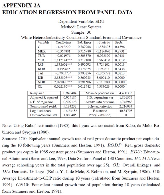
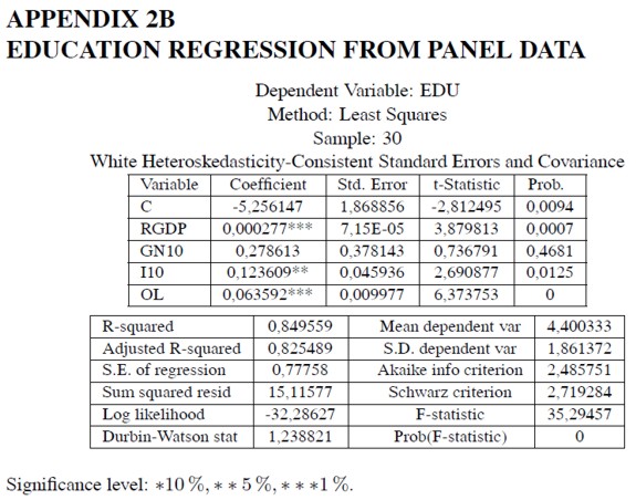
This second possibility would imply that structural transformation imposes some education requirements (Klees, 1989; Levin and Kelley, 1994; Bils and Klenow, 2000; Easterly, 2001, ch. 4). Data are not inconsistent with this hypothesis. In Appendix 2A, a regression is run for educational attainment (EDU) against the index of overall linkages (0L) and the set of country dummies (Colombia is the reference country). The coefficient associated with overall linkages is estimated positive and statistically significant at all levels; the coefficients associated with some industrialized country dummies –Yugoslavia, Japan, Israel and Norway– are estimated positive and significant. If educational attainment is run against the basic set of regressors and the overall linkages measure (Appendix 2B), the measure of overall linkages (OL) and the initial income level per capita (RGDP) exhibit the highest statistical significance level, in that order. Hence, education and economic growth might depend jointly on the measure of overall linkages.

A Cross-Country Data Set

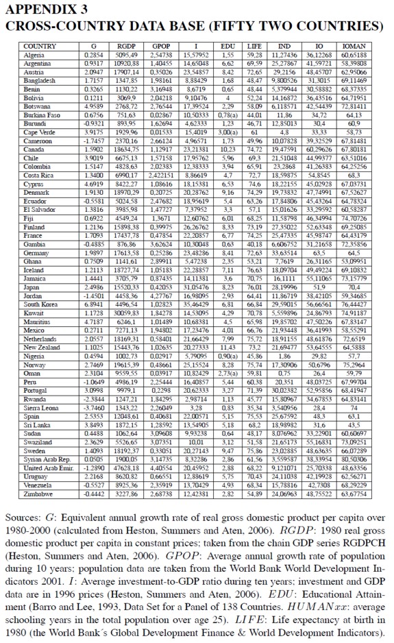
The above considerations and estimations are based on a small but representative sample of nine semi-industrial and industrial countries. Since the data set is a non-balanced panel, the results might be subject to all sorts of potential problems of endogeneity. Instead of attempting to solve them, this research project focused on the analysis of a larger cross-country data set of fifty two (52) countries (Appendix 3). Since the project aims at estimating the impact of industrialization on economic growth, three industrialization indices were built: the 1980 share of the manufacturing sector in GDP (IND), the 1980 input-output coefficient for the whole economy (IO), and the 1980 input-output coefficient for the manufacturing sector (IOMAN). The data for these indices were collected from the United Nations´ National Accounts Statistics. The year 1980 was chosen mainly because information for many less developed countries and even for developed countries is not available for previous years; thus, a previous year analysis would reduce both the sample size and the representativeness of less developed economies.

It would have been useful to have a direct measure of interindustrial linkages as in the panel data set. Since this information is not available, the project took advantage of the patterns of structural transformation that were examined before to postulate that the tightness of interindustrial linkages (and the degree of economic diversification) must be correlated with the manufacturing GDP share and the input-output coefficients for the whole economy and the manufacturing sector (I N D, I O and I O M A N). Even though cross-country differences of product composition and relative prices may affect these coefficients (As Table 3 shows, some of these coefficients are too high for the corresponding level of development), the research project used them because there was no alternative. On the other hand, an ordering of these coefficients shows that in general highly developed economies tend to exhibit higher industrialization indices.

Taking into account the shift from panel data to cross-country analysis, the methodological approach is quite similar. The dependent variable is the average growth rate of per capita GDP between 1980 and 2000; in order to estimate this variable a semi-logarithmic regression of per capita GDP against time is run for each country over the period 1980-2000. The source of GDP data is the Penn-World Table (Heston, Summers and Aten, 2006). A basic set of independent variables is defined: the per capita real gross domestic product in 1980 (RGDP), the average rate of population over the period (GPOP), the average investment rate over the period (I), and the initial educational attainment (EDU). A second set of variables include the three industrialization measures and the dummy variable for oil exporting countries.

The educational attainment variable was taken from Barro and Lee´s (1993) statistical data base. As education data for Burkina Faso, Cape Verde, Nigeria and Oman are not available for 1980, they were estimated taking advantage of the high correlation coefficient across countries between the log of educational attainment and life expectancy at birth, 89%.

Cross-Country Growth Regressions

Appendix 3 is a cross-country data base. It contains information for 52 countries of different levels of development. Using this information the growth regressions shown in Table 3 are run. As in the panel data exercises, the hypothesis of heteroscedasticity cannot be rejected at the 1 percent level. Hence, OLS estimates are corrected using White´s consistent covariance matrix.

The first regresssion includes as independent variables the basic set. All the estimated coefficients yield the expected signs, and all of them, with the exception of the log of education, are significant at the 5% level. The second and third regressions add the manufacturing share (I N D) as independent variable in a linear and a quadratic way, respectively; however, the associated coefficients are not significant. The fourth and fifth regressions use instead the aggregate input-output coefficient (I O) as independent variable; but the associated coefficients in these regressions are not significant either. The sixth and seventh regressions use the manufacturing input-output coefficient (IOMAN) as independent variable; in this case, the quadratic expression in IOMAN –seventh regression– does yield estimated coefficients which are significant at the 1% level.

Taking into account that educational attainment is estimated for four countries, they are excluded from the sample and the eighth regression is run for just 48 observations; this regression yields quite similar coefficients to the previous one, and the significance levels are practically equal. The ninth regression includes in the set of regressors the square of the average investment rate (I-SQ); the estimated coefficient is negative –as in the panel data exercises- but it is not significant. All not significant variables are dropped in the tenth regression; the result improves greatly: the estimated coefficients exhibit the expected sign: RGDP(-),GPOP(-), I(+), IOMAN(-), and IOMAN - SQ(+), and all of them are significant at the 1% level. The eleventh regression is run in order to test whether the condition of oil exporter has some effect on economic growth, but the corresponding estimated coefficient is not significant. Our preferred estimation is regression 10, for it exhibits the highest significance levels. Regressions 12 and 13 are run for the 21 higher income countries of the sample excluding oil exporting countries (Norway, Denmark, Iceland, Canada, Sweden, Netherlands, Austria, Germany, France, Finland, Japan, New Zealand, Spain, Argentina, Portugal, Uruguay, Cyprus, Mexico, Costa Rica, Chile and Mauritius). The results confirmed that in this case the relationship between the manufacturing input-output coefficient and economic growth is linear, as in the panel data exercises.

Since the cross-country regressions 7 to 11 imply that economic growth is a significant convex function in the manufacturing input-output coefficient (IOMAN), the minimum IOMAN value is estimated as follows: -α / ( 2 β), where α(< 0) is the estimated IOMAN coefficient, and β(> 0) is the estimated IOMAN2 coefficient. The IOMAN threshold estimations fluctuate slightly around the value 64 (see Table 3). This value points out the relative minimum level of industrial economic integration that must be achieved before enjoying the dynamic benefits of industrialization. This analysis implies, of course, that changes in IOMAN reflect changes in manufacturing technological integration; it would be absurd to claim that higher input-output coefficients due to relaxation of cost minimizing behaviour would lead to higher economic growth.

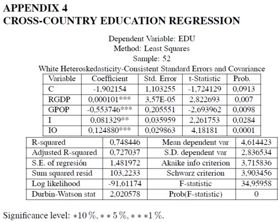
As in the panel data econometric exercises, the cross-country regressions reveal that educational attainment [log(EDU)] does not seem to be a good predictor of economic growth once one controls for manufacturing interindustrial linkages (IOMAN). However, as shown by the cross-country regression in Appendix 4, education does seem to depend on some structural factors, like real GDP (RGDP: positive and significant correlation), population growth (GPOP: negative and significant correlation), average investment rate (I: positive and marginally significant correlation), and aggregate input-output coefficient (IO: positive and highly significant correlation). The exercises revealed that the manufacturing input-output coefficient (IOMAN) is not a better predictor of educational attainment than the aggregate input-output coefficient (IO). Thus, as in the panel data exercises, aggregate measures of industrialization –the measure of overall linkages (OL) in the panel data, and the aggregate input-output coefficient (IO) in the cross-country data base– does seem to impinge positively on educational attainment levels.

SOME CONCLUDING COMMENTS

Regression analyses on a small panel data set and a larger cross-country data set are the basis for the following comments:

• Cross-country econometric analyses for the whole sample of countrieswhich includes both industrialized and non-industrialized countries do not reject the hypothesis that there exists a nonlinear –quadratic and convex– relationship between industrialization and economic growth. If this hypothesis were true it would imply that countries enjoy the benefits of industrialization in economic growth after surpassing some threshold of technological integration in the manufacturing sector.
• When the cross-country analyses are restricted to industrialized and semiindustrial countries, as in the panel data econometric analysis, the relationship between industrialization and growth seems to become linear. In these cases the econometric exercises capture mainly the dominant positive effect of industrialization on growth for sufficiently high indices of technological integration in the manufacturing sector (in other words, these analyses only capture the increasing section of the “u” relationship).
• The cross-country econometric analyses yield that technological integration in the manufacturing sector is highly correlated with economic growth, whilst aggregate technological integration is not. This result might imply that the manufacturing sector behaves as a leading sector.
• The previous features help to explain why rich (industrialized) countries tend to grow faster in the long-run than poorer countries. Corollary: the convergent effect related to initial GDP per capita is overcome by divergent effects related to industrialization.
• Economic growth is not significantly correlatedwith educational attainment when one controls for technological integration in the manufacturing sector. Two likely explanations may act together to explain this result: first, measurement error bias due to the exclusion of education quality levels (EDU is a quantitative measure of education in years); second, educational attainment might not be a determinant of economic growth, instead it might be determined by the degree of economic development.
• The latter hypothesis is not rejected by the available data sets: this paper finds a strong positive correlation between education and the measures of overall linkages (OL in the panel data regressions, IO in the cross-country regressions). If this hypothesis is true, education is revealed as a necessary but not sufficient condition for economic growth. In whatever scenario, education cannot be neglected. It provides many more external benefits than just economic growth; for instance, as seen before, education and life expectancy at birth are highly correlated.

Further analyses are required in order to test the hypothesis of an industrialization threshold for enhancing long-run economic growth. The complex relationship between education and economic growth should also be reviewed. If our hypotheses are confirmed, some policy recommendations would be appropriate. First, government economic policies aimed at increasing economic growth should enhance the process of economic diversification and structural transformation. Second, educational policies should go hand-in-hand with industrialization policies so that human capital supply matches human capital demand along the path of development.

APPENDIX 1

APPENDIX 2

APPENDIX 3

APPENDIX 4

---

REFERENCES

1. Amsden, A. (1989). Asia´s Next Giant. Londres: Oxford University Press.

2. Barro, R. J. and Lee, J.-W. (1993). International Comparisons of Educational Attainment. Journal of Monetary Economics, 32(3), 363-394.

3. Barro, R. and Sala-i-Martin, X. (1995). Economic Growth. New York: McGraw Hill.

4. Bils, M. and Klenow, P.J. (2000). Does Schooling Cause Growth?. American Economic Review, 90(5), 1160-1183.

5. Caballero, R.J. and Lyons, R.K. (1990). Internal Versus External Economies in European Industry. European Economic Review, 34, 805-830.

6. Chenery, H.B., Robinson, S. and Syrquin, M. (1986). Industrialization and Growth: A Comparative Study. Washington: World Bank.

7. Easterly, W. (2001). The Elusive Quest of Growth. Economists´ Adventures and Misadventures in the Tropics. Cambridge: MIT Press.

8. Easterly, W. and Levine, R. (2001). It´s Not Factor Accumulation: Stylized Facts and Growth Models. World Bank Economic Review, 15(2), 177-220.

9. Hall, R.E. and Jones, C.J. (1997). Levels of Economic Activity across Countries. American Economic Review Papers and Proceedings, 87(2), 173-177.

10. Heston, A., Summers, R. and Aten, B. (2006). Penn World Table Version 6.2. Philadelphia, PA: Center for InternationalComparisons of Production, Income and Prices at the University of Pennsylvania.

11. Hirschman, A.O. (1958). The Strategy of Economic Development. New Haven: Yale University Press, Inc.

12. Kaldor, N. (1961). Capital Accumulation and Economic Growth. F.A. Lutz and D. Hague (eds.), The Theory of Capital (pp. 177-222), ch. 10. Londo: Macmillan.

13. Kaldor, N. (1966). Causes of the Slow Rate of Economic Growth of the United Kingdom, An Inaugural Lecture. Cambridge: Cambridge Univ. Press.

14. Klees, S.J. (1989). The Economics of Education: A more that Slightly Jaundiced View of Where We are Now. In Francoise Caillods (ed.), Prospects for Educational Planning (pp. 244-291). Paris: UNESCO, IIEP.

15. Kubo, Y. (1985). A Cross-Country Comparison of Interindustrial Linkages and the Role of Imported Intermediate Inputs. World Development, 13(12), 1287-1298.

16. Kubo Y., Melo, J., Robinson, J., and Syrquin, M. (1986). Interdependence and Industrial Structure. In Chenery, H.B., Robinson, S. and Syrquin, M. (1986). Industrialization and Growth: A Comparative Study. Washington: World Bank, Oxford University Press..

17. Landes, D. (1998). The Wealth and Poverty of Nations. New York: W.W. Norton and Company.

18. Leontief, W. (1986). The Structure of Development. InW. Leontief, Input-Output Economics (chapter 8). Oxford: Oxford University Press.

19. Levin, H.M. and Kelley, C. (1994). Can Education Do It Alone?. Economics of Education Review, 13 (2), 97-108

20. Levine, R. and Renelt, D. (1992). A Sensitivity Analysis of Cross-Country Growth Regressions. American Economic Review, 82(4), 942-963.

21. Lucas, R. Jr. (1988). On the Mechanics of Economic Development. Journal of Monetary Economics, 22, 3-42.

22. Madisson, A. (1994). Explaining the Economic Performance of Nations, 1820-1989. In W.J. Baumol, R.R. Nelson and E.N. Wolff, (eds.), Convergence and of Productivity: Cross-National Studies and Historical Evidence. New York: Oxford University Press.

23. Matsuyama, K. (1992). Agricultural Productivity, Comparative Advantage and Economic Growth. Journal of Economic Theory, 58, 317-334.

24. Murphy, K., Shleifer, A. and Vishny, R. (1989). Industrialization and the Big Push. Journal of Political Economy, 97(5), 1003-1026.

25. Perry, G., Arias, O., Maloney, W.M., López, J.H. and Servén, L. (2006). Poverty Reduction and Growth: Virtuous and Vicious Circles. Washington: World Bank Latin American and Caribbean Studies.

26. Ortiz, C.H. (1994). Integración Tecnológica y Crecimiento Económico: Evidencia Empírica. Ensayos sobre Política Económica, 25, 73-95.

27. Ortiz, C.H. (2004). An Economic Growth Model showing Government Spending with Reference to Colombia and Learning-by- Doing. Colombian Economic Journal, 2(1), 156-188.

28. Ortiz, C.H. (2008). Aprendizaje en la Producción de Bienes de Capital, Crecimiento Acelerado y Cambio Estructural. Cuadernos de Economía, 27(48), 115-142.

29. Pritchett, L. (1997). Divergence, Big Time. Journal of Economic Perspectives, 11(3), 3-17.

30. Rebelo, S. (1991). Long-Run Policy Analysis and Long-Run Growth. Journal of Political Economy, 99(3), 500-521.

31. Rodrik, D. (2007). Industrial Development: Some Stylized Facts and Policy Directions. En United Nations, Industrial Development for the 21st Century: Sustainable Development Perspectives (pp. 7-28). New York: UN.

32. Romer, P. (1986). Increasing Returns and Long-Run Growth. Journal of Political Economy, 94(5), 1002-1037.

33. Romer, P. (1987). Growth Based on Increasing Returns Due to Specialization. American Economic Review, Papers and Proceedings. 77, 56-62.

34. Romer, P. (1990). Endogenous Technological Change. Journal of Political Economy, 98(5), S71-S102.

35. Sraffa, P. (1960). Production of Commodities by Means of Commodities. Cambridge: Cambridge University Press.

36. United Nations. (1960-1992). National Accounts Statistics: Main Aggregates and Detailed Tables. New York: UN.

37. World Bank. (2001). World Development Indicators 2001. New York: World Bank and Oxford University Press.

38. World Bank. (2000). Global Development Finance & World Development Indicators. Washington: World Bank.

39. Young, A. (1991). Learning by Doing and the Dynamic Effects of International Trade. Quarterly Journal of Economics, 106, 369-405.

40. Young, A. (1993). Invention and Bounded Learning by Doing. Journal of Political Economy, 101, 443-472.

---