Publicado
Electricity consumption forecasting using singular spectrum analysis
DOI:
https://doi.org/10.15446/dyna.v82n190.43652Palabras clave:
Electricity consumption forecasting, singular spectrum analysis, time series, power system planning (es)Descargas
DOI: https://doi.org/10.15446/dyna.v82n190.43652
Electricity consumption forecasting using singular spectrum analysis
Previsión del consumo de electricidad mediante análisis espectral singular
Moisés Lima de Menezes a, Reinaldo Castro Souza b & José Francisco Moreira Pessanha c
a Statistics Dept, Fluminense Federal University,
Niterói, Brazil. moises_lima@msn.com
b Electrical
Engineering Dept, Pontifical Catholic University of Rio de Janeiro, Rio de
Janeiro, Brazil. Reinaldo@ele.puc-rio.br
c Institute of
Mathematics and Statistics, State University of Rio de Janeiro, Rio de Janeiro,
Brazil. professorjfmp@hotmail.com
Received: May 24th, 2014. Received in revised form: December 1st, 2014. Accepted: December 12th, 2014.
This work is licensed under a Creative Commons Attribution-NonCommercial-NoDerivatives 4.0 International License.
Abstract
Singular Spectrum
Analysis (SSA) is a non-parametric technique that allows the decomposition of a
time series into signal and noise. Thus, it is a useful technique to trend
extraction, smooth and filter a time series. The effect on performance of both
Box and Jenkins' and Holt-Winters models when applied to the time series
filtered by SSA is investigated in this paper. Three different methodologies are evaluated in the SSA approach: Principal Component Analysis (PCA), Cluster Analysis and Graphical
Analysis of Singular Vectors. In order to illustrate and compare the methodologies, in
this paper, we also present the
main results of a computational experiment with the monthly residential
consumption of electricity in Brazil.
Keywords: electricity consumption forecasting, singular spectrum analysis, time series, power system planning.
Resumen
El Análisis Espectral Singular (AES) es una técnica no paramétrica que
permite la descomposición de una serie de tiempo en una componente de señal y
otra de ruido. De este modo, AES es una técnica útil para la extracción de la
tendencia, la suavización y el filtro una serie de tiempo. En este artículo se
investiga el efecto sobre el desempeño los modelos de Holt-Winters y de Box
& Jenkins al ser aplicados a una serie de tiempo filtrada por AES. Tres
diferentes metodologías son evaluadas con el enfoque de AES: Análisis de
Componentes Principales (ACP), análisis de conglomerados y análisis gráfico de
vectores singulares. Con el fin de ilustrar y comparar dichas metodologías, en
este trabajo también se presentaron los principales resultados de un
experimento computacional para el consumo residencial mensual de electricidad
en Brasil.
Palabras clave: pronóstico del consumo de electricidad, análisis espectral singular, serie de tiempo, planeamiento del sistema eléctrico.
1. Introduction
Load forecast is a requisite to all decision-making processes in the power systems operation and planning [1]. Traditionally, the load forecasts are classified in three time periods: short-term (usually half-hourly, hourly and daily forecasts up to 1 month ahead), mid-term (1 month - 5 years ahead) and long-term (5 years onwards). The short-term load forecasting [2,3] is important for the daily operation (unit commitment). The mid-term load forecasting is essential to the maintenance scheduling, hydro resources management, schedule fuel purchases, tariff setting and energy trading [4]. The long-term load forecasting signals the need to expand the capacity of the generation and transmission systems [1].
In the Brazilian electricity market, energy trading is realized through auctions where the generators compete in order to meet the demand growth at the lowest price. The auctions procedure starts with the mid/long-term monthly demand forecasts provided by the distribution utilities and ends with the energy contracts agreed between all distributors and each generator that wins the auction [5]. The energy contracting occurs one, three or five years before supply starts with contracts lasting from five to thirty years [6]. Therefore, the mid-term electricity consumption forecasts play a fundamental role in the energy auctions. The demand for electricity can be divided into several groups: residential, commercial, industrial, rural and miscellaneous. These groups grow at different rates, thus each group must be forecast separately [1].
Traditionally, Box & Jenkins and the multiple linear regression models have been considered in mid-term electricity consumption forecasting [1,4,7]. Despite the good results obtained by these methods, efforts have been made to improve them [4,8, 9]. One way to improve the performance of the mid-term forecasting methods consists in filtering the time series data [4,10]. Among the available methods able to extract the signal component from a time series, the Singular Spectrum Analysis (SSA) has been successfully applied in several scientific fields [11,12].
SSA decomposes a time series into a sum of a small number of independent components interpretable as trend, oscillatory components and noise. SSA is a method for signal processing that can be used, among other applications, for example, in smoothing and filtering [12,13]. One of the advantages of SSA is its nonparametric nature, i.e., it is not necessary to know or specify a parametric model for the time series under study. A detailed description of the theoretical and practical foundations of the SSA technique can be found in [11,12].
A good example of the benefits provided by SSA filtering can be found in [14], where forecasts are provided for the industrial production in Europe. In the context of the electric power system, [15] presents the use of SSA in the monthly affluent flow forecast, essential information to the hydropower system operation and [16] presents a geometric combination approach to forecasting residential electricity consumption. In another example, [17] proposes a model-free approach for day-ahead electricity price forecasting based on SSA and [18] presents a hybrid model combining periodic autoregressive models (PAR(p)) and SSA.
In [4] the Spanish peninsular monthly electric consumption time series is split into two components: the trend and the fluctuation around it. After that, a neural network is trained to forecast each component separately. These predictions are added up to obtain an overall forecasting. The authors show that the results obtained are better than those reached when only one neural network was used to forecast the original consumption series.
This paper investigates the use of SSA in mid-term forecasting of the monthly electricity consumption for the residential class. In Brazil, the residential class is responsible for approximately 26% of the total electricity consumption and represents 85% of the consumers. This paper shows similar results related to [14], but considering three approaches in SSA before fitting the ARIMA and Holt-Winters models. Both results confirm that SSA improves the accuracy of forecasting.
The remainder of this article is organized as follows: Section 2 has a description of the SSA methods, while the traditional predictive methods are presented in Section 3. The computational experiment is presented in Section 4 and the results and discussion are reported in Section 5. Finally, in section 6 the main conclusions are drawn.
2. Singular spectrum analysis
The basic version of the SSA method has two steps: decomposition and reconstruction.
2.1. Decomposition
The decomposition step involves two stages: embedding and singular value decomposition (SVD).
Embedding is a procedure in
which a time series  is mapped into a sequence of lagged vectors
  ,
in which
  ,
for all
  ,
where
  and L takes
any integer value in the range
  .
.
The matrix  is known as trajectory matrix [14] and the
parameter L is the window length of
the trajectory matrix [11].
The trajectory matrix X can be expanded via singular value decomposition as (1):

where ,
and the set
  correspond to the eigenvalues of the positive
semidefinite matrix
  taken in order of magnitude and
  denotes the respective eigenvectors. According
to [12],
 .
.
Let d be the rank of the trajectory matrix X(i.e., the number of nonzero eigenvalues), then the identity described in (1) can be rewritten as:

where 
The collection  is called eigentriple of SVD of the trajectory matrix X. The contribution of
each component in (1) can be measured by the ratio of singular values, given by
  for each l.
2.2. Reconstruction
The reconstruction step also has two stages: grouping and diagonal averaging.
Grouping is a procedure that
groups the elementary matrices into  disjoint groups and adding the matrices within
each group. Let
  be the set of indices of the
  elementary matrices classified in a same group
i. Then the matrix corresponding to the group i is defined as:
  , so the identity (2) can be rewritten as:

The contribution of the component  can be measured by the ratio of singular
values given by:

Consider the trajectory matrix  and assume that
  and
and . Consider that
  is an
element in the line
  and column
  of matrix
  . The element
  of SSA
component
  is
computed by the Diagonal Averaging procedure applied to the matrix
  .
.
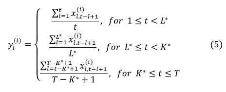
Each
SSA component  concentrates part of the energy of the
original series
  which can
be measured by the ratio of singular values (4). According to [12], the SSA
component
  can be
classified into three categories: trend, harmonic components (cycle and
seasonality) and noise.
2.3. Separability
Separability is one of the leading concepts in SSA [20].
This property characterizes how well the different components are separated
from each other. A good measure of separability is the weighted correlation
(w-correlation), a function that quantifies the linear dependence between two
SSA components  and
and  :
:
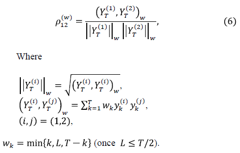
The separability allows for a statistical check of whether two SSA components are well separated in terms of linear dependence. The matrix containing the absolute values of the w-correlations corresponding to the full decomposition can provide useful information for grouping the eigentriples [17]. If the absolute value of w-correlation is small, so the SSA components are classified as w-orthogonal (or quasi w-orthogonal) otherwise, they are said to be poorly separated. It is a useful concept in the SSA grouping stage [17].
2.4. Choice of optimal value of L
The question of the optimal value of  remains open. [19], illustrates a long
discussion about the ideal value of window length assuming that this value can
be fixed or variable. In several cases, the general recommendation is to choose
the window length at slightly less than half the size of the series:
  .
In [20], the suitable value of L is
  According to [21], the choice of
  depends on several criteria including
complexity of the data, the aim of the analysis and the forecasting horizon. In
[21], the authors show a new bound of
  for the multivariate case and study the
optimum value for the number of eigenvalues
  to choose. By selecting
  smaller than the true number of eigenvalues,
some parts of the signal(s) will be lost, and then the reconstructed series
becomes less accurate. However, if one takes
  greater than the value that it should be, then
noise is included in the reconstructed series. Although, considerable attempts
have been made and various techniques considered for selecting the optimal
values of
  and
and  in SSA, there is not enough theoretical
justification for choosing these parameters. In addition, if the series has a
seasonal behavior with monthly periodicity, it is advisable to choose
reasonably large values of
  (but smaller than
  .
In this paper the optimum value of
  is obtained by testing values from
  to
to  and performing the BDS test [22] applied to
the noise series after decomposition.
3. Predictive methods
This section presents the Holt-Winters and ARIMA models; both traditionally used in mid-term consumption prediction.
3.1. Holt-Winters models
According to [23], exponential
smoothing methods are based on the assumption that the data are weighted
differently. Usually, recent observations contain more relevant information
than older ones, so that the weighting of the data (time series) decreases exponentially
as the observation becomes older. A particular case of exponential smoothing
method is the multiplicative Holt-Winters method, which performs modeling
dynamically (i.e. with time-varying parameters) its components: level ,
trend
 )
and seasonality
 :
:

where  is a
stochastic error,
  is the
observed value at time
  and
and  is the
seasonal factor in
  relative to
month m. The family
  of seasonal
factors, where
  is the set
of months of the year that satisfy the constraint
 , where
  is the size
of the seasonal cycle. In the process of estimating the parameters of equation
(7), three hyperparameters (time invariant quantities) are used, denoted by
a, β and l which are associated, respectively, to the estimates
of level, trend and seasonality and whose optimal values are in the cube
 . Recently, [24] has compared the forecasts for
the exponential smoothing and neural networks and removed trend and seasonality
using seasonal differentiation.
3.2. Box-Jenkins models
A second order stationary stochastic process is defined as
a family  of random variables whose moments (mean,
variance and covariance) are time invariants for all t. Consider the sequence
  as a realization of
  .
Box & Jenkins [23] proposes the following linear equation for
  .
.

where  is a stochastic error and
  is the observed value in
  .
For seasonal time series, the following formulation is used:

The fitting of such SARIMA model to monthly seasonal time series is carried out in four stages; structural identification, parameters estimation, goodness of fit tests and forecasting. For details, see [23].
4. Case study
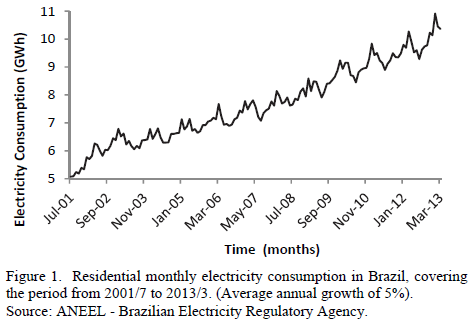
For the computational experiment, we considered the monthly time series of the residential electricity consumption in Brazil shown in Fig. 1. The time series covers the period from July 2001 to March 2013 (141 observations). In this period, the series experienced an average growth of approximately 5%. The length of the in sample period is 129 and the out of sample is 12. The computational implementation was carried out with different software: MATLAB, for the SSA approach via principal component analysis in the SVD; Caterpillar SSA [25], for detailed verification of SSA filtering via graphical analysis of singular vectors via their scatter plots and the periodogram analysis; E-Views, for the analyzes of BDS tests (independence) [26] and ARIMA models [27]; Forecast Pro for Windows for Holt-Winters modeling; R, to apply SSA using hierarchical clustering [28], and Microsoft Excel to generate graphs.
5. Results and discussions
In this study, three SSA filtering approaches were applied: principal component analysis under SVD (PCA-SVD) [28], cluster analysis integrated with PCA-SVD [29] and graphical analysis of singular vectors of SVD [30]. Each filtering approach generated a smoothed time series of the monthly residential electricity consumption which was modeled by two predictive methods: ARIMA and Multiplicative Holt-Winters.
5.1. Principal component analysis under SVD (PCA-SVD)
In the PCA-SVD approach, an optimal window length L is defined for trajectory matrix X and an integer N such that the SVD can be rewritten as:

Through diagonal averaging procedure, these sequences of
elementary matrices in (10) generate  (less noisy than the original series
  )
and
)
and  (the noise), respectively, such that the
original time series
  can be written as:

The goal of this approach is to obtain a smoothed time
series  less noisy than the original time series
  [23].
[23].
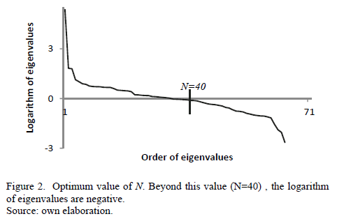
In [31], the best values of L and N using this approach were obtained following the completion of many rounds of BDS testing for several values of these parameter. In this paper, the optimum values using the same procedure are 71 and 40 respectively. Fig. 2 shows the logarithm of the 71 eigenvalues arranged in a decreasing partial order and the point defined by the optimal value of N.
In the PCA-SVD, the first 40 eigenvectors cover the signal  and the last 31 remaining eigenvectors, the
noise
 .
Removing
  in (11), one obtains the filtered series
  generated by the approach PCA-SVD such that
 .
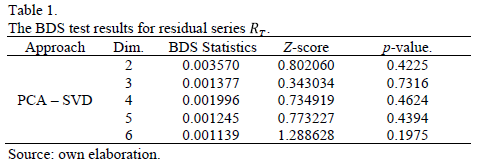
Table 1 shows the results of the BDS test applied to
 .
.
In Table 1, one can see that the null hypothesis of
independence of the BDS test is not rejected at the 5% level. So there is no
empirical evidence that the time series noise  has any structure of temporal dependence.
Based on the BDS test, one can see that the Brazilian residential electricity
consumption time series can be smoothed by
  .
.
5.2. Cluster Analysis
As before, in the
first step, the trajectory matrix X is obtained from  through
embedding with optimum window length equal to 71. In this way, 71 singular
vectors are obtained and the 31 less significant singular vectors were
classified as noise, based on the BDS test using a 5% significance level, and
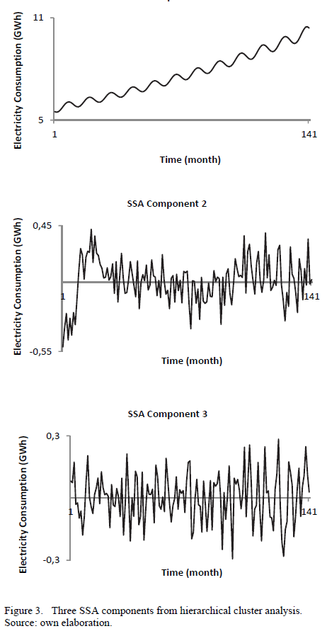
were removed. Next, the 40 remaining singular vectors were grouped into 3 SSA
components by hierarchical clustering analysis, as seen in Table 2. The
implementation of this method was carried out by the general agglomerative
hierarchical clustering in a R package called RSSA [32]. Initially, a matrix of
dissimilarities for the
  eigentriples of SVD was generated. Next, each
object was assigned to its own cluster and then the algorithm proceeded
iteratively, joining, at each stage, the two most similar clusters, continuing
until three clusters were obtained. At each stage, Euclidean distances between
clusters were recomputed using the Lance-Williams dissimilarity update formula
[33].
Fig. 3 shows the plot of three SSA components obtained
from the three clusters. The BDS test is applied to each SSA component in order
to identify the noisy component. The aim of this approach is to obtain a less
noisy time series ,
by removing the noisy component.
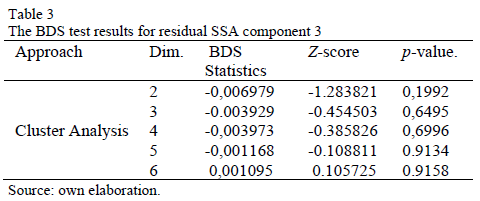
According to the BDS test in Table 3, the SSA component 3 is classified as a noisy component.
5.3. Graphical analysis of singular vectors
Analysis
of time series coordinates on the basis defined by the singular vectors
resulting from SVD identifies the components of trend, seasonality and noise
present in a time series .
The general problem consists in identifying and separating the oscillatory
components from those that are part of the trend. According to [12], the
graphical analysis of such coordinates in pairs
allows us to visually identify the harmonic components of the series.
Similarly to the computational experiments above, the
optimal window length was considered as  ,
but with an optimal truncation
  ,
generating 50 singular vectors. The software used for this approach was
Caterpillar SSA [25]. Through graphical analysis of pairs of singular vectors
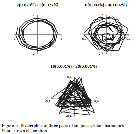
it is possible to classify them according to their behavior. Consider a pure
harmonic with frequency equal to
  ,
phase equal to
  ,
amplitude equal to
  and period
  defined as a divisor of window length L and K. If the parameter
  assumes an integer value, then
  is classified as a harmonic period [14]. The
sine and cosine functions having equal frequencies, amplitudes and phases
generate a scatter plot, which displays a circular pattern [12]. Thus, the
scatter diagram shows a regular polygon with
  vertices. For a frequency
  with m and n integers and primes, the points are vertices of a regular polygon
of n vertices [12]. Thus, the
identification of components that are generated by a harmonic analysis can be
performed by the pictorial analysis of the patterns determined by different
pairs of components.
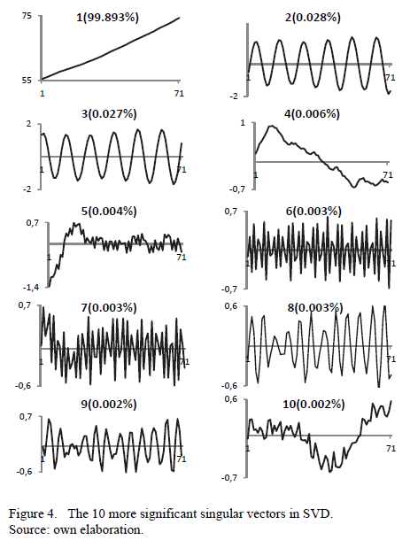
Fig. 4 shows the ten first singular vectors. One can see that components 1, 4, 5 and 10 correspond to the trend. It is possible to identify that components 2, 3, 6 - 9 are harmonic components.
For the other components in Fig. 4, there is no need for a deeper analysis. The first component (trend) accounts for nearly all the variability present in the time series. The domain of the trend component can be explained by the growth of the Brazilian population and the respective growth of the number of households [34]. Additionally, Brazil has experienced an improvement in income distribution, which allowed greater diffusion of home appliances, as well as the efforts to meet the universal access to electricity, expected for the year 2015. The result of classical decomposition of this series presents similar values of trend (95.83%), seasonal (2.77%) and noise (1.40%).
Fig. 5 shows three pairs of singular vectors, it is found that the singular vectors 2 and 3 are harmonic components with period equal to 12 months, while the singular vectors 8 and 9 are harmonic components with period equal to 6 months. In turn, the singular vectors 19 and 20 are harmonic components with period equal to 3 months.
The periodogram
analysis helps in the identification of a general harmonic component. The
periodogram of the singular vector of each eigentriple provides information
about the periodic behavior of the component and frequency (period) of the
oscillations. Therefore, proper grouping can be made with the help of the
periodogram analysis. For the series , the periodogram
  is defined
as

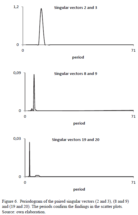
For the periodic components, the periodogram has sharp spikes around the component's frequency (period). Hence the visual identification is straightforward. Fig. 6 shows the respective periodogram associated to scatterplots of Fig. 5:
By exclusion, the singular vectors that are not classified as trend component or harmonic component via graphical analysis are classified as noise. After graphical analysis of the 50 singular vectors of the SVD, the classification shown in Table 4 was obtained.
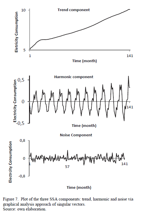
Fig. 7 shows the plot of the three SSA components obtained by graphical analysis in the reconstruction phase where the elementary matrices are grouped into three groups generating the components in SVD. Note that the trend component captures a slight change in trend after 15 months and the noisy component captures the highest difference between the original time series and the smoothed times series at the 57th month.
Table 5 shows the weighted correlation matrix among the three components identified by graphical analysis of the singular vectors. According to the figures presented in Table 5, the three components look well separable.
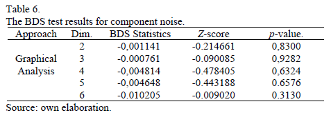
According to the BDS test in Table 6, one can see that the noisy component does not present time dependence structure. Therefore, this component can be classified as a noise.
In the PCA-SVD method (equation 11), the components aren't separated in trend, harmonic and noise, but rather in signal and noise. In this approach many noisy components are still part of the signal. In Table 2 obtained by the cluster analysis, one can see that the eigentriples 2 and 3 are added to the trend component, but the periodogram analysis (Fig. 6) shows that these eigentriples are part of a harmonic component. Similarly, the cluster analysis classifies the eigenvectors 11 - 18 as harmonic component, but they are noise components (see Table 4) obtained by graphical analysis of the singular vectors. The results above show that the graphical analysis of a singular vector is a more effective method to classify SSA eigentriples.
5.4. Forecasting models
After identifying the noisy components by the three methods under study (PCA-SVD, Cluster Analysis and Graphical Analysis of Singular Vectors), these components are extracted from the original time series resulting in smoothed time series. Thus, there are four time series to be modeled: the original and three filtered time series via SSA.
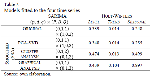
In the specification of the  model with
 ,
it is necessary to choose the lags
  the degree of differencing d and D. It is considered that the best SARIMA model minimizes the
Bayesian Information Criterion (BIC) [35]. The best Holt-Winters' model (HW)
also minimizes the BIC with linear trend and multiplicative seasonality. The
models are shown in Table 7.
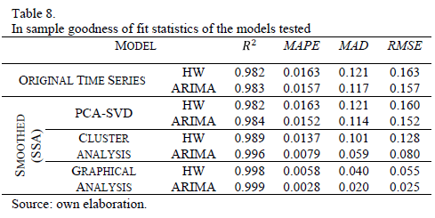
To check the predictive power of the SSA approach applied
to the electricity consumption time series, Table 8 shows the in sample results
of the goodness of fit statistics:  ,
mean absolute percentage error (MAPE),
mean absolute deviation (MAD), and
root-mean-square error (RMSE). One can see that the values of MAPE, MAD, and RMSE using the SSA approach are lesser than these values for the
original time series.
The out of sample 1-step ahead error statistics are shown in Table 9. Note that the graphic analysis is also the best approach of SSA filtering.
6. Conclusions
Three alternatives
to remove the noisy component of a time series by SSA method were proposed in
this paper. The method was applied to a real time series corresponding
to monthly residential electricity consumption in Brazil. Among the three
alternatives evaluated the graphical analysis of singular vector is the more
effective method to remove the noisy component. In the sequence, the
Holt-Winters and Box- Jenkins were applied to the original and filtered time
series obtained by SSA. The in-sample and out-of-sample goodness of fit
statistics (MAPE, MAD and RMSE) obtained for the eight fitted models, show that
the SSA method with graphical analysis of singular vectors also provided the
more accurate forecasts. This approach provides a more detailed analysis of the
components, thus, the results tend to be better. In addition, the best value of  corresponds to
  and the BDS test proved effective in
identifying the noise components.
References
[1] Wang, X. and McDonald, J.R., Modern power system planning. McGraw Hill, 1994.
[2] Gross, G. and Galiana, F., Short-term load forecasting. Proceedings of the IEEE. 75 (12), pp. 1558-1573, 1987. DOI: 10.1109/PROC.1987.13927.
[3] Santos, P.J., Martins, A., Pires, A., Martins, J., and Mendes, R., Short-term load forecast using trend information. International Journal of Energy Research, 30 (10), pp. 811-822, 2006. DOI: 10.1002/er.1187.
[4] Gonzalez-Romera, E., Jaramillo-Morán, M.A., and Carmona-Fernandez, D., Monthly electric energy demand forecasting based on trend extraction. IEEE Transactions on power systems, 21 (4), pp. 1946-1953, 2006. DOI: 10.1109/TPWRS.2006.883666.
[5] Barroso, L.A., Street, A., Granville, S., and Bezerra, B., Bidding strategies in auctions for long-term electricity supply contracts for new capacity. Power and Energy Society General Meeting - Conversion and Delivery of Electrical Energy in the 21th Century, Pittsburgh, 2008.
[6] Castro, C.M.B., Marcato, A.L.M., Silva, I.C.S., Dias, B.H., Silva Jr, G.E., and Oliveira, E.J., Brazilian energy auctions analysis based on evolutionary algorithms. IEEE Bucharest Power Tech Conference, Bucharest, Rumania, 2009.
[7] Abdel-Al, R.E. and Al-Garni, A.Z., Forecasting monthly electric energy consumption in Eastern Saudi Arabia using univariate time-series analysis. Energy, 22 (11), pp. 1059-1069, 1997. DOI: 10.1016/S0360-5442(97)00032-7.
[8] Falvo, M.C., Lamedica, R., Pierazzo, S., and Prudenzi, A., A knowledge based system for medium term load forecasting, transmission and distribution Conference and Exhibition, IEEE PES, Dallas, USA, 2006.
[9] Borlea, I., Buta, A. and Lustrea, B., Some aspects concerning mid-term monthly load forecasting using ANN, EUROCON 2005 - The International Conference on 'Computer as a Tool', Belgrade, Serbia, 2005.
[10] Broomhead, D.S. and King, G.P., Extracting qualitative dynamics from exponential data. Physica D. 20 (2-3), pp. 217-236, 1986. DOI: 10.1016/0167-2789(86)90031-X.
[11] Elsner, J.B. and Tsonis, A.A., Singular spectrum analysis. A new tool in time series analysis. Plenum Press, 1996.
[12] Golyandina, N., Nekrutkin, V. and Zhigljavsky, A. ,Analysis of time series structure: SSA and related techniques. Chapman & Hall/CRC New York, 2001.
[13] Hassani, H., Heravi, S. and Zhigljavsky, A., Forecasting UK industrial production with multivariate singular spectrum analysis, in The 2012 International Conference on the Singular Spectrum Analysis and its Applications, Beijing, China, 2012.
[14] Hassani, H., Heravi, S. and Zhigljavsky, A., Forecasting European industrial production with singular spectrum analysis. International Journal of Forecasting. 25 (1), pp. 103-118, 2009. DOI: 10.1016/j.ijforecast.2008.09.007.
[15] Cassiano, K.M., Junior, L.A.T, Souza, R.M., Menezes, M.L., Pessanha J.F.M. and Souza, R.C., Hydroelectric energy forecast. International Journal of Energy and Statistics, 1 (3), pp. 205-214, 2013. DOI: 10.1142/S2335680413500142.
[16] Junior , L.A.T., Menezes, M.L., Cassiano, K.M., Pessanha, J.F.M. and Souza, R.C., Residential electricity consumption forecasting using a geometric combination approach. International Journal of Energy and Statistics, 1 (2), pp. 113-125, 2013. DOI: 10.1142/S2335680413500087.
[17] Miranian, A., Abdollahzade, M. and Hassani H., Day-ahead electricity price analysis and forecasting by singular spectrum analysis. IET Generation, Transmission & Distribution, 7 (4), pp. 337-346, 2013. DOI: 10.1049/iet-gtd.2012.0263.
[18] Menezes, M.L., Souza, R.C., and Pessanha, J.F.M., Combining singular spectrum analysis and PAR(p) structures to model wind speed time series. Journal of Systems Science and Complexity, 27 (1), pp. 29-46, 2014. DOI: 10.1007/s11424-014-3301-8.
[19] Golyandina, N., On the choice of parameters in singular spectrum analysis and related subspace-based methods. Statistics and Its Interface, 3, pp. 259-279, 2010.
[20] Golyandina, N. and Vlassieva, E,. First-order SSA-errors for long time series: Model examples of simple noisy signals. In Proceedings of 6th St. Petersburg Workshop on Simulation, 1, St. Petersbusg State University, St. Petersburg, Rusia, pp. 314-319, 2009.
[21] Hassani, H., Mahmoudvand, R. and Zokaei, M., Separability and window length in singular spectrum analysis. Comptes Rendus Mathematique, 349 (17-18), pp. 987-990, 2011. DOI: 10.1016/j.crma.2011.07.012.
[22] Brock, W.A., Dechert, W., Scheinkman, J. and LeBaron, B., A test for independence based on the correlation dimension. Econometric reviews, 15 (3), pp. 197-235, 1996.
[23] Box, G.E.P. and Jenkins, G.M., Time series analysis: Forecasting and control. Holden-Day, 1970.
[24] Velásquez-Henao, J.D., Zambrano-Perez, C.O. and Franco-Cardona, C.J., A comparison of exponential smoothing and neural networks in time series prediction. DYNA, 80 (182), pp. 66-73, 2013.
[25] Gistat Group. Caterpillar SSA. Petersburg University, Department of Mathematics, Russia, 2010. [Online]. Available at: http://www.gistatgroup.com/cat/index.html
[26] Lin, K., The ABC's of BDS. Journal of computational intelligence in finance, 97 (jul/Aug.). pp. 23-26, 1997.
[27] Chatfield, C., The Analysis of time series: An introduction, 6th ed., Chapman & Hall/CRC, 2003.
[28] Danilov, D. and Zhigljavsky, A., Principal components of time series: The caterpillar method. University of St. Petersburg Press, Rusia 1997.
[29] Aldenderfer, M.S. and Blashfield, R.K., Cluster analysis. Sage publications, California, USA, 1984.
[30] Hassani, H. and Mahmoudvand, R., Multivariate singular spectrum analysis: A general view and new vector forecasting approach. International Journal of Energy and Statistics, 1 (1), pp. 55-83. 2013. DOI: 10.1142/S2335680413500051.
[31] Hassani, H., Singular spectrum analysis: Methodology and comparison. Journal of Data Science, 5, pp. 239-257, 2007.
[32] Golyandina, N. and Korobeynikov, A., Basic singular spectrum analysis and forecasting with R. Computational Statistics & Data Analysis, 71, pp. 934-954, 2014.
[33] Lance, G.N. and Williams, W.T., A general theory of classificatory sorting strategies, I. Hierarchical Systems. Computer J. 9, pp. 373-380, 1966.
[34] Pessanha, J.F.M. and Leon N., Long-term forecasting of household and residential electric customers in Brazil. IEEE Latin America Transactions, 10 (2), pp. 1537-1543, 2012.
[35] Schwarz, G., Estimating the dimension of a model. The Annals of Statistics, 6 (2), pp. 461-464. March, 1978.
M.L. Menezes, received a Dr in Electrical Engineering from Pontifical Catholic University of Rio de Janeiro (PUC-Rio), Brazil. He is a professor of Statistics at Fluminense Federal University (UFF), Brazil and his research interests are in time series analysis, singular spectrum analysis and applied statistics. ORCID: 0000-0002-2233-0137.
R.C. Souza received a PhD in Bayesian forecasting from Warwick University, UK. Presently, he is a full professor in statistics and time series analysis at Pontifical Catholic University of Rio de Janeiro (PUC-Rio), Brazil and his research interests are in the area of forecasting with applications to the energy market.
J.F.M. Pessanha, received a Dr degree in Electrical Engineering from Pontifical Catholic University of Rio de Janeiro (PUC-Rio), Brazil. He is a professor at State University of Rio de Janeiro (UERJ) Brazil and teaches courses on statistics, econometrics and multivariate data analysis. As a researcher, his interests include the application of statistical and optimization methods in power systems economics, power system reliability; short and long term electrical load forecasting.
Cómo citar
IEEE
ACM
ACS
APA
ABNT
Chicago
Harvard
MLA
Turabian
Vancouver
Descargar cita
CrossRef Cited-by
1. Halit Apaydin, Mohammad Taghi Sattari, Kambiz Falsafian, Ramendra Prasad. (2021). Artificial intelligence modelling integrated with Singular Spectral analysis and Seasonal-Trend decomposition using Loess approaches for streamflow predictions. Journal of Hydrology, 600, p.126506. https://doi.org/10.1016/j.jhydrol.2021.126506.
2. Sourav Kumar Mukhopadhyay, Michael Zara, Irene Telias, Lu Chen, Remi Coudroy, Takeshi Yoshida, Laurent Brochard, Sridhar Krishnan. (2020). A Singular Spectrum Analysis-Based Data-Driven Technique for the Removal of Cardiogenic Oscillations in Esophageal Pressure Signals. IEEE Journal of Translational Engineering in Health and Medicine, 8, p.1. https://doi.org/10.1109/JTEHM.2020.3012926.
3. Sourav Kumar Mukhopadhyay, Sridhar Krishnan. (2020). A singular spectrum analysis-based model-free electrocardiogram denoising technique. Computer Methods and Programs in Biomedicine, 188, p.105304. https://doi.org/10.1016/j.cmpb.2019.105304.
4. Bogdan Dima, Ştefana Maria Dima. (2017). Energy consumption synchronization between Europe, United States and Japan: A spectral analysis assessment. Renewable and Sustainable Energy Reviews, 77, p.1261. https://doi.org/10.1016/j.rser.2017.03.042.
5. Amelia Dewi Masyitoh, Etik Zukhronah, Isnandar Slamet. (2022). Forecasting for monthly rainfall in Gondang Reservoir Lamongan using Singular Spectrum Analysis (SSA) method. INTERNATIONAL CONFERENCE ON SCIENCE AND APPLIED SCIENCE (ICSAS) 2021. INTERNATIONAL CONFERENCE ON SCIENCE AND APPLIED SCIENCE (ICSAS) 2021. 2391, p.020003. https://doi.org/10.1063/5.0075313.
6. Keila Mara Cassiano, Moisés Lima de Menezes, Reinaldo Castro Souza, José Francisco Moreira Pessanha. (2017). Introducing DBSCAN in the singular spectrum analysis procedure. International Journal of Energy and Statistics, 05(02), p.1750009. https://doi.org/10.1142/S2335680417500090.
7. Paula Maçaira, Rainer Elsland, Fernando Cyrino Oliveira, Reinaldo Souza, Gláucia Fernandes. (2020). Forecasting residential electricity consumption: a bottom-up approach for Brazil by region. Energy Efficiency, 13(5), p.911. https://doi.org/10.1007/s12053-020-09860-w.
8. Paul A. Adedeji, Stephen Akinlabi, Oluseyi Ajayi, Nkosinathi Madushele. (2019). Non-linear autoregressive neural network (NARNET) with SSA filtering for a university energy consumption forecast. Procedia Manufacturing, 33, p.176. https://doi.org/10.1016/j.promfg.2019.04.022.
9. Ammar H. Elsheikh, Amal I. Saba, Hitesh Panchal, Sengottaiyan Shanmugan, Naser A. Alsaleh, Mahmoud Ahmadein. (2021). Artificial Intelligence for Forecasting the Prevalence of COVID-19 Pandemic: An Overview. Healthcare, 9(12), p.1614. https://doi.org/10.3390/healthcare9121614.
Dimensions
PlumX
Visitas a la página del resumen del artículo
Descargas
Licencia
Derechos de autor 2015 DYNA

Esta obra está bajo una licencia internacional Creative Commons Atribución-NoComercial-SinDerivadas 4.0.
El autor o autores de un artículo aceptado para publicación en cualquiera de las revistas editadas por la facultad de Minas cederán la totalidad de los derechos patrimoniales a la Universidad Nacional de Colombia de manera gratuita, dentro de los cuáles se incluyen: el derecho a editar, publicar, reproducir y distribuir tanto en medios impresos como digitales, además de incluir en artículo en índices internacionales y/o bases de datos, de igual manera, se faculta a la editorial para utilizar las imágenes, tablas y/o cualquier material gráfico presentado en el artículo para el diseño de carátulas o posters de la misma revista.


