Published
Nonlinear forecasting of stream flows using a chaotic approach and artificial neural networks
Keywords:
Kızılırmak, k-nearest neighbor, and feed-forward neural networks, mutual information function, correlation dimension (en)
This paper evaluates the forecasting performance of two nonlinear models, k-nearest neighbor (kNN) and feed-forward neural networks (FFNN), using stream flow data of the Kızılırmak River, the longest river in Turkey. For the kNN model, the required parameters are delay time, number of nearest neigh- bors and embedding dimension. The optimal delay time was obtained with the mutual information function; the number of nearest neighbors was obtained with the optimization process that minimi- zes RMSE as a function of the neighbor number and the embedding dimension was obtained with the correlation dimension method. The correlation dimension of the Kızılırmak River was d = 2.702, which was used in forming the input structure of the FFNN. The nearest integer above the correlation dimension (i.e., 3) provided the minimal number of required variables to characterize the system, and the maximum number of required variables was obtained with the nearest integer above the value 2d + 1 (Takens, 1981) (i.e., 7). Two FFNN models were developed that incorporate 3 and 7 lagged discharge values and the predicted performance compared to that of the kNN model. The results showed that the kNN model was superior to the FFNN model in stream flow forecasting. However, as a result from the kNN model structure, the model failed in the prediction of peak values. Additionally, it was found that the correlation dimension (if it existed) could successfully be used in time series where the determina- tion of the input structure is difficult because of high inter-dependency, as in stream flow time series.
Resumen
Este trabajo evalúa el desempeño de pronóstico de dos modelos no lineares, de método de clasificación no paramétrico kNN y de redes neuronales con alimentación avanzada (FNNN), usando datos de flujo del río Kizilirmak, el mayor de Turquía. Para el modelo kNN, los parámetros requeridos son tiempo de retraso, número de vecindarios cercanos y dimensión de encrustamiento. El tiempo óptimo de retraso fue obtenido con la función de información mutua; el número de vecindarios cercanos fue obtenido con la optimización de procesos que minimizan el RMSE como una función del número de vecindarios y la dimensión de incrus- tación fue obtenida con el método de dimensión correlativa. La dimensión de correlación del río Kizilirmak fue utilizado en la formación de la estructura de ingreso de las redes FFNN. La integración cercana sobre la dimensión de correlación proveyó el número mínimo de variables requeridas para caracterizar el sistema y el número máximo de variables requeridas fue obtenido con el número entero por encima del valor (Takens, 1981). Se desarrollaron dos modelos de redes FNNN que incorporan 3 y 7 valores de descargas retrasadas y el desempeño de predicción comparado con el modelo kNN. Los resultados muestran que el modelo kNN fue superior al modelo de redes FFNN en el flujo de pronósticos. Sin embargo, como un resultado del modelo de estructura kNN, el modelo falla en los valores pico. Adicionalmente, se encontró que la dimensión de correla- ción (de existir) podría ser usada eficientemente en series temporales donde la determinación de estructura de ingreso es difícil por la gran interdependencia, como en las series temporales de flujo.
FLUID DYNAMICS
Nonlinear forecasting of stream flows using a chaotic approach and artificial neural networks
Hakan Tongal
Engineering Faculty, Civil Engineering Department, Süleyman Demirel University, Turkey
Manuscript received: 11/02/2013
Accepted for publication: 01/11/2013
ABSTRACT
This paper evaluates the forecasting performance of two nonlinear models, k-nearest neighbor (kNN) and feed-forward neural networks (FFNN), using stream flow data of the Kızılırmak River, the longest river in Turkey. For the kNN model, the required parameters are delay time, number of nearest neighbors and embedding dimension. The optimal delay time was obtained with the mutual information function; the number of nearest neighbors was obtained with the optimization process that minimizes RMSE as a function of the neighbor number and the embedding dimension was obtained with the correlation dimension method. The correlation dimension of the Kızılırmak River was d = 2.702, which was used in forming the input structure of the FFNN. The nearest integer above the correlation dimension (i.e., 3) provided the minimal number of required variables to characterize the system, and the maximum number of required variables was obtained with the nearest integer above the value 2d + 1 (Takens, 1981) (i.e., 7). Two FFNN models were developed that incorporate 3 and 7 lagged discharge values and the predicted performance compared to that of the kNN model. The results showed that the kNN model was superior to the FFNN model in stream flow forecasting. However, as a result from the kNN model structure, the model failed in the prediction of peak values. Additionally, it was found that the correlation dimension (if it existed) could successfully be used in time series where the determination of the input structure is difficult because of high inter-dependency, as in stream flow time series.
Key words: Kızılırmak, k-nearest neighbor, feed-forward neural networks, mutual information function, correlation dimension
RESUMEN
Este trabajo evalúa el desempeño de pronóstico de dos modelos no lineares, de método de clasificación no paramétrico kNN y de redes neuronales con alimentación avanzada (FNNN), usando datos de flujo del río Kizilirmak, el mayor de Turquía. Para el modelo kNN, los parámetros requeridos son tiempo de retraso, número de vecindarios cercanos y dimensión de encrustamiento. El tiempo óptimo de retraso fue obtenido con la función de información mutua; el número de vecindarios cercanos fue obtenido con la optimización de procesos que minimizan el RMSE como una función del número de vecindarios y la dimensión de incrustación fue obtenida con el método de dimensión correlativa. La dimensión de correlación del río Kizilirmak fue utilizado en la formación de la estructura de ingreso de las redes FFNN. La integración cercana sobre la dimensión de correlación proveyó el número mínimo de variables requeridas para caracterizar el sistema y el número máximo de variables requeridas fue obtenido con el número entero por encima del valor (Takens, 1981). Se desarrollaron dos modelos de redes FNNN que incorporan 3 y 7 valores de descargas retrasadas y el desempeño de predicción comparado con el modelo kNN. Los resultados muestran que el modelo kNN fue superior al modelo de redes FFNN en el flujo de pronósticos. Sin embargo, como un resultado del modelo de estructura kNN, el modelo falla en los valores pico. Adicionalmente, se encontró que la dimensión de correlación (de existir) podría ser usada eficientemente en series temporales donde la determinación de estructura de ingreso es difícil por la gran interdependencia, como en las series temporales de flujo.
Palabras clave: Kizilirmak, método de clasificación no paramétrico kNN, redes neuronales con alimentación avanzada, funciones de información mutua, dimensión de correlación.
1. Introduction
Reliable and accurate stream flow forecasting is essential for water resources management. Stream flow simulations and forecasts are also important for optimization of water resources planning and allocation. Therefore, in addition to many other reasons, understanding stream flow dynamics constitutes one of the most important problems in hydrology and water resources. For this purpose, many data-driven models have been developed, including linear, nonlinear, parametric and nonparametric models for hydrologic time series prediction in the past decades (Marques et al., 2006). Generally, in regard to system dynamics, there are two basic assumptions that underlie different modeling techniques, stochastic and chaotic dynamics. Regarding the former assumption, the observed hydrologic time series originated from a stochastic process with an infinite number of degrees of freedom. To this assumption, the mean behavior of a time series could be captured with linear models such as autoregressive, autoregressive moving-average (Al-Awadhi and Jolliffe, 1998; Toth et al., 2000), autoregressive integrated moving-average (Chang et al., 2002; Lisi and Villi, 2001) and seasonal autoregressive integrated moving-average (Modarres, 2007; Ooms and Franses, 2001; Pekárová et al., 2009), from which great results have been obtained. However, to utilize these models, a priori assumptions are required, such as stationarity and Gaussian distribution. As most hydrological time series involve non-stationarity and non-Gaussian conditions, the data should be transformed before it can be used in stochastic models. However, after this transformation, nonlinearity still exists, and time series are processed with a linearity assumption (Chen et al., 2008). Recent studies have shown that the complex nonlinear behavior of stream flow dynamics should not necessarily be the outcome of a stochastic process. With the advent of deterministic chaos theory, a few hydrologic modeling studies have suggested irregular behavior could be the outcome of simple deterministic systems influenced by a few nonlinear interdependent variables (Khokhlov et al., 2008; Sivakumar, 2003; Yu et al., 2011). Numerous researchers have tried to reveal chaotic behavior in hydrologic time series, such as river flow (Ng et al., 2007; Sivakumar, 2007; Sivakumar et al., 2001), lake level (Frison et al., 1999; Khokhlov et al., 2008) and rainfall (Dhanya and Kumar, 2011; Sivakumar et al., 2006). Because the studies revealed possible chaotic behavior in stream flow dynamics, the requisition for chaotic prediction methods in stream flow was obvious. The most employed prediction method for chaotic hydrological time series is the k-nearest neighbor (k-NN), which was used in this study (Elshorbagy et al., 2002; Liu et al., 1998; Sivakumar, 2003; Wu et al., 2009). However, in the hydrology literature, the studies that compare the modeling capability of the k-NN approach with other nonlinear modeling techniques are limited. To obtain more insight into the modeling capability of k-NN, another widely used nonlinear modeling technique the feed-forward neural network (FFNN) (Araghinejad et al., 2011; Deka et al., 2012; Kuo-Lin, 2011; Vafakhah, 2012; Wu and Chau, 2010) was employed. Additionally, in determining the number of input parameters for FFNN, to the author's knowledge, the chaotic procedure in this study is the first proposed. The values for the dominant variables obtained from the chaos analysis were used as the minimum and maximum input parameters in the FFNN.
Generally, the prediction techniques for a dynamic system can generally be divided into two approaches: local and global (Wu and Chau, 2010). Because the local approach uses only nearby states to make predictions, the k-nearest neighbor can be included in this class, and FFNN can be classified as the latter one. Therefore, in this study, we preliminarily evaluate which nonlinear approach, local or global, is more efficient in forecasting stream flow time series. The two nonlinear approaches' modeling capabilities are compared for the Kızılırmak River, the longest river in Turkey. The paper is organized as follows. Section 2 introduces the study area and the stream flow time series that are used. In Section 3, the basic principles of the k-NN and the feed-forward neural network as a sub-class of ANN are described. Following this, in Section 4, the obtained results are given with a detailed discussion. The conclusions of the paper are presented in Section 5.
2. Study area and data
The Kızılırmak River basin is located between 37°58'-41°44' North latitudes and 32°48'-38°22' East longitudes. The Kızılırmak River flows through a 1,355 km long course, the longest in Turkey. In the basin, the continental climate is dominant, for which summers are characterized with moderate precipitation and winters are characterized with severe cold. The annual mean precipitation and temperature are 446.1 mm and 13.7°C, respectively. The flow regime of the river is irregular resulting from rainfall and snow-melt. The lowest discharges are observed between July and February, and the river starts to rise in the beginning of March and reaches its highest level in April (Çakmak et al., 2007). The data that were used cover the period of January 1960 to September 2004 (Figure 1), and the main statistical parameters of the stream flow time series are given in Table 1.


3. Methodology
3.1. k-Nearest Neighbor Approach
The temporal evolution of a system can be described by a multi-dimensional phase space. The most frequently used reconstruction method for a univariate or multivariate time series is the delay time method which was developed by Packard et al. (1980) and Takens (1981). The main idea behind phase-space reconstruction is that the system is characterized by self-interaction, and the observed time series can hold the information about the dynamics of the entire system (Sivakumar et al., 2002). The past observations can be embedded in an m-dimensional state space according to:

where j = 1,2,...,N—(m—1) , m is the embedding dimension of the Yj vector and is the delay time. To characterize a dynamic system with an attractor dimension d, (m > 2d + 1)-dimensional space is required (Takens, 1981). However, Abarbanel et al. (1990) proposed that m > d would be sufficient. As it is seen in Eq. (1), the main parameters that should be determined in the phase-space reconstruction method are the delay and the embedding dimension parameters. The most commonly used methods for determining these parameters are the mutual information (MI) and the correlation dimension methods, respectively. Another commonly used method for determining the delay parameter is the autocorrelation function (ACF). However, because the ACF does not measure the nonlinear dependence, in this study, we employed a MI function that was based on joint probabilities that enabled us to measure the nonlinear dependency beyond linear correlation. The mutual information was computed according to:

where Xi and Xi- are successive values, and P(Xi) and P(Xi-) are the individual probabilities of Xi and Xi-, respectively and P(Xi,Xi-) is the joint probability density. To determine the optimal delay time parameter, it is advised to use the local minimum of the MI (Frazer and Swinney, 1986), i.e., no increase or decrease in the mutual information function's successive values for a specific lag time. However, in some MI functions, it is rather difficult to determine a local minimum. Therefore, to determine the optimal delay time, we recommend using the following formula to amplify the successive differences between the calculated MI function values (Tongal et al., 2013):

where MIcurrent is the mutual information value of which relative change will be calculated, MInext is the successive value of MIcurrent The first local minimum could be taken where the relative change of mutual information as a function of delay time started to become constant with lag time.
With a properly selected time delay, the considered time series can be reconstructed in the m-dimensional phase space by calculating the correlation exponent from the correlation integral (C(r)) as follows:

where H is the Heaviside step function with H(u) = 1 for u > 0, and H(u) = 0 for u < 0, u = r - ║Yi - Yj║, r is the radius of a sphere centered on Yi or Yj, ║·║ is the Euclidean norm, and N is the number of data points. C(r) gives the probability of two randomly selected vectors that lie within a certain distance (Ng et al., 2007). The dimension d of the state space is related to the correlation integral as:

Additionally, the logarithm of both sides of Eq. (5) gives a linear relationship where the slope equals to the correlation exponent d. If the correlation exponents increase as a function of embedding dimension, then the considered system can be thought of as stochastic, otherwise it is chaotic. In the latter situation, the correlation exponents reach a saturation value, which provides the correlation dimension of the system. The correlation dimension is a parameter that gives the number of dominant processes that are acting in the system dynamics (Sivakumar and Jayawardena, 2002). With the determination of the optimal delay time and embedding dimension, the state space of the system can be constructed, from which interpreting the dynamics of an m-dimensional map ƒ(·) is possible using the following equation:

where et is a noise term and Y(t) and Y(t+T) are vectors of dimension m that describe the state of the system at times t (current state) and t+T (future state), respectively. If the function ƒ(·) is known, it is possible to predict the future trajectory of a system. The ƒ(·) function can be found with the k-nearest neighbor (k-NN) approach which was proposed by Farmer and Sidorowich (1987). In this approach, the nearby states are used to obtain future forecasts. One of the most commonly used functions for k-NN is the weighted form:

where ai(t) are the nearest neighbors of the last observed value (i.e., prediction starting point) and ( L)i are the weights to be adjusted using the information from the n-nearest points. L denotes that these weights are different for each forecasted point. For more details, please refer to Wu and Chau (2010), Ng et al. (2007), Laio et al., (2003) and Liu et al. (1998).
3.2. Feed-Forward Neural Networks
Artificial neural networks (ANN) use a multilayered approach that approximates complex mathematical functions to process data. An ANN is a system that is composed of discrete layers with each layer including at least one neuron. With a connection weight, each node of a layer is connected to the node(s) of the preceding layer but not to nodes of the same layer (Sahoo et al., 2009). Considering the feed forward neural network architecture in Figure 2, if the layers and the neurons in the layers increase, the architecture of the ANN becomes more complex, which complicates the solution process. Therefore, it is important to select an optimal ANN architecture. In this study, the numbers of neurons in the layers were determined with a trial and error process that minimized the root mean square error calculated from the differences between the predicted and observed values.

In Figure 2, the input signal propagates from layer to layer through the network in a forward direction. The weight vectors between the layers (Wij and Wjk) were randomly generated in the range between -1 and 1. The total output of a jth hidden neuron was computed according to:

where  is the value of the ith input parameter to the hidden layer neurons, bj is the bias for the jth hidden layer neuron and n is the total number of input neurons. The calculated total input signal, Sj, that received the jth hidden layer neuron was converted to an output signal using an activation function φj. The output signal of the jth hidden layer neuron was φj[Sj(n)] for the n th pattern of the training data set. The output neuron received signals from all hidden-layer neurons and converted them to a single signal as output using an activation function φk[·]. Thus, the input and output signal of the kth output neuron were, respectively:

where bk is the bias and N is the total number of neurons in the hidden layer (Sahoo et al., 2009). By comparing the estimated output with the desired output, the weights were adjusted with well-known error propagation algorithms including Levenberg-Marquardt (LM), Bayesian regularization (BR) and Gradient descent with momentum and adaptive learning rate back-propagation algorithm (GDX). In this study, we employed the LM algorithm as a learning algorithm. Detailed information about the LM algorithm can be found elsewhere (Aqil et al., 2007; Daliakopoulos et al., 2005). In this study, the Tangent Sigmoid transfer function, of which the validity has been proven in hydrological applications, was used:

where u is the Sj and Sk in the hidden layer and output layer, respectively.
3.3. Performance Indices
To evaluate the model performances, the following performance indices were used; Nash-Sutcliffe Coefficient of Efficiency (CE), Mean Absolute Error (MAE), Persistence Index (PI), Root Mean Square Error (RMSE), Relative Volume Error (RVE) and Coefficient of Determination (R2). Nash and Sutcliffe (1970) proposed the coefficient of efficiency in the following form:

where Oi and Pi are the observed and predicted values, respectively, and Ō is the mean value of the observed values. Mean absolute error is a measure that evaluates the absolute deviation of the predicted values from the observed ones. It is calculated as:
The Persistence Index (PI) proposed by Kitanidis and Bras (1980), compares the predictions of a model with the best estimate for the future, which is given by the last observation (Randrianasolo et al., 2011). The index has the following form:

where Oi-L is the last observed value at time i minus the lead time L. RMSE is one of the most widely used criterions to assess model efficiency, and it evaluates the forecast errors with the following form:

Because this criterion is sensitive to large forecast errors (i.e., the errors are amplified by squaring), it provides a good measure for the goodness-of-fit at high flows. Additionally, it has the same units as the observed values; thus, it enables the interpretation of the magnitude of error. The RVE criterion shows the total relative error resulting from the model predictions as:
R2 describes the proportion of the total variance in the observed data that can be explained by the model and is formulated as below:

R2 changes between 0 (no relation) and 1 (perfect fit), which describes how much of the observed dispersion is explained by the model.
4. Results and discussion
To determine the chaotic dynamics within the stream flows, the correlation dimension method was applied. To calculate the correlation integrals, the delay time () was computed using the mutual information function and its relative change with lag time (Figure 3).

In Figure 3, it was difficult to select the first local minimum from the original MI function. The amplified differences (i.e., the relative change of the MI) between the successive values were more informative about where the first local minimum could be found. In the MI relative change, the mutual information function was stable and fluctuated around a constant value after 30 days. By determining the delay value, the correlation integrals were computed by the Grassberger-Procaccia algorithm for different embedding dimensions (m) from m = 1 to m = 25 (Figure 4a).

From the scaling regions (i.e., nearly linear sections of each integral plots) of the calculated correlation integrals, the correlation exponents were calculated with the least squares estimation method and each calculated correlation exponent was plotted against its embedding dimension as seen in Figure 4b. Because the correlation exponent values increased with the embedding dimension up to a certain value (i.e. d = 2.702) and then fluctuated around this value, chaotic behavior was indicated. This value was the correlation dimension calculated for the Kızılırmak River and the nearest integer above this value provided the minimum embedding dimension for reconstructing the phase-space or the number of variables (i.e., the number of dominant variables) necessary to model the dynamics of the system (Khokhlov et al., 2008; Sivakumar and Jayawardena, 2002; Stehlik, 1999). Thus, the results from these analyses showed that the required minimum number of variables to model the system dynamics was 3 (3 > 2.702) and the maximum number of variables to model the system dynamics was 7 (7 > (2d + 1)). In the k-NN model development, the embedding dimension was taken as 3 by considering the required minimum embedding dimension obtained from the above analysis. The required nearest neighbor numbers for k-NN analysis was determined with a trial and error process that minimized RMSE as a function of nearest neighbor number. Figure 5 shows that the RMSE decreased as a function of nearest neighbor number until nearest neighbor number equaled 33 days and after this value, RMSE started to increase. Therefore, the optimal nearest neighbor number was selected as 33 days.

With these results, the required parameters for the k-NN model were obtained. To determine whether the obtained correlation dimension could be used as the lag value for the discharges, the following model structures were built. To the author' knowledge, this study was the first to take the correlation dimension as the of required lag value for the discharges. By considering the correlation dimension value as the required number of variables that characterize the system, the following FFNN model structures were constructed that incorporate a minimum of 3 (3 > 2.702) and maximum of 7 (7 > (2d + 1)) lagged values.
Typically, the training data set is selected as 70%-80% of a time series and the remaining part is used as the calibration and test period (Banerjee et al., 2011; Daliakopoulos et al., 2005; Riad et al., 2004). In this study, approximately 78% (36 years) of the entire data set was selected as the training period, and the remaining part, approximately 22% (10 years), was selected for the test period.

The FFNN model structures contained one input layer, two hidden layers and one output layer. The number of neurons in the hidden layers was determined using an optimization process that minimized RMSE as a function of the number of neurons (Figure 6). The results from these models are given in Figure 7.

From Figure 7, the inadequacy of the k-NN model is obvious; failing to capture the peak flows. The reason for this is that the k-NN model predicted the next value by considering the past observed values as much as the number of nearest neighbors. To obtain accurate peak flow prediction, the number of peak values in the past observed period should be as much as the nearest neighbor number. If the number of observations of peak flow in the training period is smaller than the nearest neighbor number, than the model fails in the accurate prediction of peak flows. This is also valid for low flow predictions. From Figure 7, there is a section at the end of the test period in which no flow was observed. The k-NN model constantly over-predicted this period. However, the FFNN models performed better in peak flow predictions than the k-NN model. To acquire more insight into the models' performance, the performance indices were calculated and are given in Table 3.

By means of the performance indices, the best model was selected as the k-NN model and the worst model was selected as the FFNN-I model. The highest PI, CE and R2 and the lowest RMSE, RVE and MAE values were obtained with the k-NN model. As the results showed, there was not much difference between the CE and R2 values, and stand-alone evaluation of these performance indices does not give much insight into the model comparison. In addition to these criteria, RMSE, RVE, MAE and PI demonstrated the clear superiority (nearly twice as much) of the k-NN model over the FFNN model. Therefore, in the model comparison, it was important to take into account other performance indices that emphasized different features of the predicted values.
These results showed that the correlation dimension could be used in the determination of the FFNN model structure by taking the lagged values as the minimum and maximum dominant variable number. To the authors' knowledge, this study is the first to show that the correlation dimension could be used in determining of number of lagged values of the discharges. This is important where the autocorrelation function remains high for higher lags such as in this case (Figure 8).
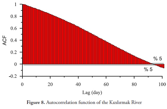
It is difficult to determine the optimal lag values in the model structure where the autocorrelation function values start to become statistically insignificant. For instance, in Figure 8, the autocorrelation function becomes statistically insignificant on the 90th day. To determine the optimal lag values that will be considered in the model structure, various models should be considered that incorporate combinations of lag values up to 90. Obviously, this is quite time consuming. However, by considering the correlation dimension of the examined system, it is possible to construct two models that incorporate minimum and maximum lagged values that are determined from the correlation dimension. This result is evidence that chaos theory could be used in simplifying the modeling procedure, in which the determination of the input structure is rather difficult.
5. Conclusions
Hydrological systems are complex and dynamic in nature as their current and future states depend on numerous variables (Tongal et al., 2013). Therefore, it is important to determine the number of dominant variables acting within the system dynamics. In regards to this, the methods from chaos theory provided us a proper framework. In this study, one of the chaotic forecasting methods, the k-NN method, was employed for the Kızılırmak River, the longest river in Turkey. The necessary parameters for this method are the delay time, the embedding dimension and the nearest neighbor number. The optimal delay time was determined from the mutual information function and the nearest neighbor number was determined from the optimization process that minimized RMSE as a function of the nearest neighbor number. In determining the optimal delay time from the MI function, we calculated the relative differences between the successive values of the MI function. The optimal delay time was selected as 30 days. To determine the embedding dimension for the k-NN method, the correlation integrals were calculated for various embedding dimensions, i.e., m = 1 to m = 25. When the obtained correlation exponents from the correlation integrals were plotted as a function of the embedding dimension, the correlation exponents reached a value (correlation dimension, d = 2.702), which gave us the dimension of the system. The dimension of the system shows the number of dominant variables that are acting within the system dynamics. For this system, the minimal number of dominant variables was 3 (3 > 2.702) and the maximum was 7 (7 > (2d + 1)). To the author' knowledge, this study is the first to examine whether the obtained correlation dimension could be used in the model development phase. In feed-forward neural network input parameter determination, the two models (FFNN-I and FFNN-II) that were described incorporated lagged discharge values of 3 and 7, respectively. The number of hidden layer neurons was determined from a trial and error process that minimized RMSE. The predictions obtained from the models showed that the k-NN model, which is one of the most commonly used chaotic prediction approaches, was superior to the FFNN models, which are a sub-class of another nonlinear prediction approach, the artificial neural networks. However, the k-NN model failed to predict the peak flows, in which the FFNN demonstrated better performance. Therefore, the k-NN model (with averaging method) should not be used, when peak flow forecasting is important. Additionally, the results showed that the correlation dimension method can successfully be used instead of the time-consuming trial and error process to determine input parameters for ANN, where the interdependency of time series is high.
References
Abarbanel, H.D.I., Brown, R. and Kadtke, J.B., (1990). Prediction in chaotic nonlinear systems: Methods for time series with broadband Fourier spectra. Physical Review A, 41: 1782-1807.
Al-Awadhi, S. and Jolliffe, I., (1998). Time Series Modelling of Surface Pressure Data. International Journal of Climatology, 18: 443-455.
Aqil, M., Kita, I., Yano, A. and Nishiyama, S., (2007). A comparative study of artificial neural networks and neuro-fuzzy in continuous modeling of the daily and hourly behaviour of runoff. Journal of Hydrology, 337(1–2): 22-34.
Araghinejad, S., Azmi, M. and Kholghi, M., (2011). Application of artificial neural network ensembles in probabilistic hydrological forecasting. Journal of Hydrology, 407(1-4): 94-104.
Banerjee, P., Singh, V.S., Chatttopadhyay, K., Chandra, P.C. and Singh, B., (2011). Artificial neural network model as a potential alternative for groundwater salinity forecasting. Journal of Hydrology, 398(3–4): 212-220.
Chang, F.J., Chang, L.-C. and Huang, H.-L., (2002). Real-time recurrent learning neural network for stream-flow forecasting. Hydrological Processes, 16(13): 2577-2588.
Chen, C.S., Liu, C.H. and Su, H.C., (2008). A nonlinear time series analysis using two-stage genetic algorithms for streamflow forecasting. Hydrological Processes, 22: 3697-3711.
Çakmak, B., Kendirli, B. and Ucar, Y., (2007). Evaluation of Agricultural Water Use: A Case Study for Kizilirmak. Journal of Tekirdag Agricultural Faculty, 4(2): 175-185.
Daliakopoulos, I.N., Coulibaly, P. and Tsanis, I.K., (2005). Groundwater level forecasting using artificial neural networks. Journal of Hydrology, 309(1–4): 229-240.
Deka, P.C., Haque, L. and Banhatti, A.G., (2012). Discrete wavelet-Ann approach in time series flow forecasting-a case study of Brahmaputra river. International Journal of Earth Sciences and Engineering, 5(4): 673-685.
Dhanya, C.T. and Kumar, D.N., (2011). Multivariate nonlinear ensemble prediction of daily chaotic rainfall with climate inputs. Journal of Hydrology, 403: 292-306.
Elshorbagy, A., Simonovic, S.P. and Panu, U.S., (2002). Estimation of missing streamflow data using principles of chaos theory. Journal of Hydrology, 255(1–4): 123-133.
Farmer, D.J. and Sidorowich, J.J., (1987). Predicting chaotic time series. Physical Review Letters, 59: 845-848.
Frazer, A.M. and Swinney, H.L., (1986). Independent coordinates for strange attractors from mutual information. Physical Review A, 33(2): 1134–1140.
Frison, T., Abarbanel, H., Earle, M., Schultz, J. and Sheerer, W., (1999). Chaos and predictability in ocean water level measurements. . Journal of Geophysical Research Oceans, 104: 7935-7951.
Khokhlov, V., Glushkov, A., Loboda, N., Serbov, N. and Zhurbenko, K., (2008). Signatures of low-dimensional chaos in hourly water level measurements at coastal site of Mariupol, Ukraine. Stochastic Environmental Research and Risk Assessment 22: 777-787.
Kitanidis, P.K. and Bras, R.L., (1980). Real-time forecasting with a conceptual hydrologic model 2. Applications and results,. Water Resources Research, 16: 1034-1044.
Kuo-Lin, H., (2011). Hydrologic forecasting using artificial neural networks: A Bayesian sequential Monte Carlo approach. Journal of Hydroinformatics, 13(1): 25-35.
Laio, F., Porporato, A., Revelli, R. and Ridolfi, L., (2003). A comparison of nonlinear flood forecasting methods. Water Resources Research, 39(5): 1129.
Lisi, F. and Villi, V., (2001). Chaotic forecasting of discharge time series: a case study. Journal of the American Water Resources Association, 37(2): 271-279.
Liu, Q., Islam, S., Rodriguez-Iturbe, I. and Le, Y., (1998). Phase-space analysis of daily streamflow: characterization and prediction. Advances in Water Resources, 21(6): 463-475.
Marques, C.A.F. et al., (2006). Singular spectrum analysis and forecasting of hydrological time series. Physics and Chemistry of the Earth, Parts A/B/C, 31(18): 1172-1179.
Modarres, R., (2007). Streamflow drought time series forecasting. Stochastic Environmental Research and Risk Assessment, 21(3): 223-233.
Nash, J.E. and Sutcliffe, J.V., (1970). River flow forecasting through conceptual models, Part I- A discussion of principles. Journal of Hydrology, 10: 282-290.
Ng, W.W., Panu, U.S. and Lennox, W.C., (2007). Chaos based analytical techniques for daily extreme hydrological observations. Journal of Hydrology, 342: 17-41.
Ooms, M. and Franses, P.H., (2001). A seasonal periodic long memory model for monthly river flows. Environmental Modelling & Software, 16: 559-569.
Packard, N.H., Crutchfield, J.P., Farmer, J.D. and R.S., S., (1980). Geometry from a time series. Physical Review Letters 45(9): 712–716.
Pekárová, P., Onderka, M., Pekár, J., Rončák, P. and Miklánek, P., (2009). Prediction of water quality in the Danube River under extreme hydrological and temperature conditions. Journal of Hydrology and Hydromechanics, 57(1): 3-15.
Randrianasolo, A., Ramos, M.H. and Andréassian, V., (2011). Hydrological ensemble forecasting at ungauged basins: using neighbour catchments for model setup and updating. Adv. Geosci., 29: 1-11.
Riad, S., Mania, J., Bouchaou, L. and Najjar, Y., (2004). Rainfall-Runoff Model Using an Artificial Neural Network Approach. Mathematical and Computer Modelling 40: 839–846.
Sahoo, G.B., Schladow, S.G. and Reuter, J.E., (2009). Forecasting stream water temperature using regression analysis, artificial neural network, and chaotic non-linear dynamic models. Journal of Hydrology, 378(3–4): 325-342.
Sivakumar, B., (2003). Forecasting monthly streamflow dynamics in the western United States: a nonlinear dynamical approach. Environmental Modelling & Software, 18(8-9): 721-728.
Sivakumar, B., (2007). Nonlinear determinism in river flow: prediction as a possible indicator. Earth Surface Processes and Landforms(32): 969-979.
Sivakumar, B., Berndtsson, R. and Persson, M., (2001). Monthly runoff prediction using phase space reconstruction. Hydrological sciences journal, 46(3): 377-388.
Sivakumar, B. and Jayawardena, A.W., (2002). An investigation of the presence of low-dimensional chaotic behaviour in the sediment transport phenomenon. Hydrological Sciences Journal, 47(3): 405-416.
Sivakumar, B., Jayawardena, A.W. and Fernando, T.M.K.G., (2002). River flow forecasting: use of phase-space reconstruction and artificial neural networks approaches. Journal of Hydrology, 265(1-4): 225-245.
Sivakumar, B. et al., (2006). Nonlinear analysis of rainfall dynamics in California's Sacramento Valley. Hydrological Processes, 20: 1723-1736.
Stehlik, J., (1999). Deterministic chaos in runoff series. Journal of Hydrology and Hydromechanics, 47(4): 271-287.
Takens, F., (1981). Detecting strange attractors in turbulence. In: D.A. Rand, Jung, L.S. (Editor), Dynamical Systems and Turbulence, Lecture Notes in Mathematics. Springer-Verlag, Berlin, pp. 366-381.
Tongal, H., Demirel, M.C. and Booij, M.J., (2013). Seasonality of low flows and dominant processes in the Rhine River. Stochastic Environmental Research and Risk Assessment, 27(2): 489-503.
Toth, E., Brath, A. and Montanari, A., (2000). Comparison of short-term rainfall prediction models for real-time flood forecasting. Journal of Hydrology, 239(1–4): 132-147.
Vafakhah, M., (2012). Application of artificial neural networks and adaptive neuro-fuzzy inference system models to short-term streamflow forecasting. Canadian Journal of Civil Engineering, 39(4): 402-414.
Wu, C.L. and Chau, K.W., (2010). Data-driven models for monthly streamflow time series prediction. Engineering Applications of Artificial Intelligence, 23: 1350-1367.
Wu, C.L., Chau, K.W. and Li, Y.S., (2009). Predicting monthly streamflow using data-driven models coupled with data-preprocessing techniques. Water Resour. Res., 45(8): W08432.
Yu, B., Huang, C., Liu, Z., Wang, H. and Wang, L., (2011). A chaotic analysis on air pollution index change over past 10 years in Lanzhou, northwest China. Stochastic Environmental Research and Risk Assessment, 25: 643-653.
How to Cite
APA
ACM
ACS
ABNT
Chicago
Harvard
IEEE
MLA
Turabian
Vancouver
Download Citation
Article abstract page views
Downloads
License
Earth Sciences Research Journal holds a Creative Commons Attribution license.
You are free to:
Share — copy and redistribute the material in any medium or format
Adapt — remix, transform, and build upon the material for any purpose, even commercially.
The licensor cannot revoke these freedoms as long as you follow the license terms.
The Earth Sciences Research Journal is the copyright holder for these license attributes.