MOMENTO

Introduction

Quantum electrodynamics establishes a constraint on the rest mass of photon which is proposed to be zero. However, in nonzero photon mass could exist a low level that the present experiments cannot reach. The uncertainty principle establishes that the photon mass could be estimate as Μ_γ ≈ in the magnitude of about 10^-66 g as the age of the universe is about 10¹⁰ years. Although such infinitesimal mass is extremely difficult to be detected, a massive QED is not only simpler theoretically than the standard theory ^[1], it also provides a fairly solid framework for analyzing the far reaching implications of the existence of a massive photon which would have for physics. Actually, some of these possible effects, such as variation of the speed of light ^[2], the deviations of Coulomb's law ^[3] and Ampere's law ^[4], the existence of longitudinal electromagnetic waves ^[5], and the additional Yukawa potential of magnetic dipole fields ^[6,7], were seriously studied.

The massive electrodynamics or Proca's electrodynamics is the simplest model in which the photon has a small mass. Proca's electromagnetic field theory can be constructed in a unique way by adding a mass term to the Lagrangian for the electromagnetic field, namely, the Proca field is described by the following lagrangian density,

with . The parameter M can be interpreted as the photon rest mass. In this spirit, the characteristic scaling length M-1 becomes the reduced Compton wavelength of the photon, which is the effective range of the electromagnetic interaction. Nevertheless, the mass term violates gauge invariance of the theory. Cornwall [8] showed that in the Jackiw-Johnson model [9] is not possible to add a symmetry breaking mass without destroying renormalizability because the term violates the Ward identity. However, the gauge invariance can be recovered if a nonlocal, nonpolynomial terms is added to the Lagrangian which is invariance gauge in a restricted sense.

In this work we are going to follow the Cornwall procedure and recover the gauge invariance of the Proca theory. We will study in a consistent way the canonical constraint structure of the theory following the Dirac's procedure [10,11]. We determine the Hamiltonian that generates the evolution of the system and considers the full gauge freedom. Appropriated gauge conditions will be deduced in order to calculate the Dirac brackets.

However, the mail goal of Dirac's method is to obtain the Dirac brackets, which are the bridge to the commutators in quantum theory. With the categorization of the constraints as first or second class, primary or secondary, this formalism has become one of the standards for the analysis of constrained theories. Nevertheless, Faddeev and Jackiw [12] proposed a geometric method for the symplectic quantization of constrained systems. This method is based on Darboux's theorem [13] in which we do not need to introduce primary constraints as in the Dirac formalism. Also, the classification of the constraints is not necessary in this method, since all the constraints are held to the same standard [14-16].

The essential point of the symplectic quantization method is to make the system into a first order Lagrangian with some auxiliary fields, but the method does not depend on how the auxiliary fields are introduced to make the first order Lagrangian [12,13]. The first order Lagrangian, which consists of some symplectic variables and their generalized canonical momenta, gives the geometric structure of the manifold through the symplectic two form matrix. The classification of the system as constrained or unconstrained in the first order Faddeev-Jackiw formalism depends on the singular behavior of the symplectic two form matrix.

In this work we are going to study the symplectic quantization Proca's electrodynamics deriving the generalized symplectic brackets and showing that they are equivalents to the Dirac brackets.

Structure of Constraints

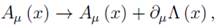
The Proca field which is described by (1) is no gauge invariance, however, it is possible to add certain nonlocal, nonpolynomial term to (1) which guarantees gauge invariance. If the transformation

is performed on the mass term, we obtain

Now, we are going to replace the gauge parameter in the following way,

Thus, we define the mass term

which is invariant under the following gauge transformations:

as long as δ2θ ≠ 0. Here, θ (x) is an auxiliar escalar field and e is a coupling constant. Thus, we come to the following effective gauge invariance Lagrangian density:

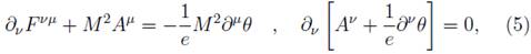
From (4), we find the Euler-Lagrange equations

and the canonical momenta associated to the fields Aν and θ are:

respectively. Then, from (6) we get the set of dynamics relation dynamical relation,

and one primary constraints [10,11],

The canonical Hamiltonian is given by

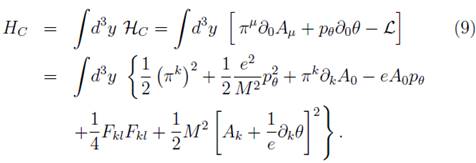
Following the Dirac's procedure [10,11], we define the primary Hamiltonian HP adding to the canonical Hamiltonian the primary constraints with their respective Lagrange multipliers

where u1 is the multipliers related to the electromagnetic constraints. The fundamental Poisson brackets (PB) between the variables of the phase space (Λμ,θ,πν,ρθ) are,

The Dirac's procedure [10,11] tell us that the primary constraints must be preserved in time (consistence condition) under time evolution generated by the primary Hamiltonian by requiring that they have a weakly vanishing PB with HP. Thus, such requirement on the constraints (8) yields

i.e., the consistence condition of Ω1 gives a secondary constraint Ω2 which is associated with the Gauss's law of the theory. It is easy to verify that there are not further constraints generated from the consistence condition of the Gauss's law because it is automatically conserved,

Then, there are not more constraints and (8) and (12) constitute the full set of constraints of the theory.

Constraint classification and gauge condition

The constraints Ω1 and Ω2 have vanishing PB among them, therefore, they are first class constraint [10,11]. Here we are in position to write the total Hamiltonian

where u2 is de Lagrange multiplier associated to the secondary first class constraint Ω2. Now, we are able to calculate the canonical equations of the system for the variables (Λμ,θ,πν,ρθ). For Λμ we have the equations

which just means that the canonical variable Αμ is defined as a linear combination of the still arbitrary Lagrange multipliers. The Hamiltonian equations for the momenta πμ are given by,

The time evolution of the dynamical variables of the scalar field are:

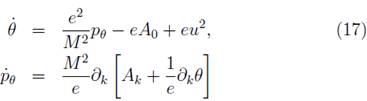
From (15), (16) and (17) it is easy to obtain

These equations are compatible with the Lagrangian field equations (5) only if suitable gauge conditions are chosen in order to eliminate the Lagrange multiplier u2.

At this stage we consider the set of first-class constraints Ω1 and Ω2, that must be considered as generators of gauge transformations. Our objective is to use the gauge freedom in our system to fix two components of Αν so that the first class constraints become second class. The problem of choosing proper gauge conditions has to be solved to fully eliminate the redundant variables of the theory at the classical level and, therefore, to proceed with a consistent quantization of the theory. Since π0 ≈ 0, one logical choice is to set:

The second gauge gauge fixing condition can be determined by closely inspect the Euler Lagrange equations of the system [17].

Thus, if we look for the ν = 0 component of the (18) equation, it produces

Then, the equation (20) will hold for all time only if:

Thus, (12) is similar to a secondary constraint following from the gauge constraint, therefore, it can be considered like the second gauge condition.

Dirac Brackets

The next step is to calculate Dirac Brackets for the set of ten constraints of the theory. The set of the first class constraints and their gauge fixing conditions, defines as:

constitute a set of second class constraints. With (22), we can construct the matrix of PB with elements:

and with the following matricial representation:

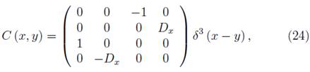
where .The inverse of the matrix is calculated from the following relationship,

Imposing the boundary condition that the fields vanish at infinity, we can find that the in inverse of (23) exists and takes the form

With this inverse we are able to define the first Dirac Brackets for two observables A (x) and B (x) [10,11],

This definition implies the elimination of the second-class constrains and the definition of an extended Hamiltonian where Ωi are strongly zero. Under the definition of Dirac brackets, the constraints (22) are strongly zero, i.e.,

The relation (28) determines that Ak and Πk could be considered as independent variables of the theory, therefore, the Dirac brackets associated to them may be computed from (27) to be

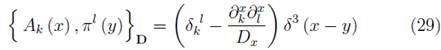
Now, using the relations (28) we can deduce the other set of DB, i.e.:

Under the definition of the Dirac brackets, the Hamiltonian which determines the evolution of the system in the reduced phase space is

Symplectic analysis for the Proca's electrodynamics

The initial set of symplectic variables defining the extended space is given by the set , and so the starting Lagrangian density is written in first order as follow [12,13] ¹:

where the zero iterated symplectic potential has the following form:

Using the initial set of symplectic variables , we have from (32) the canonical momenta

Then, we obtain the zero iterated symplectic two-form matrix defined by

with the components

The symplectic matrix is singular and it has a zero mode

where vAo (x) is an arbitrary function. From this nontrivial zero-mode, we have the following constraint

With vAo (x) arbitrary, the constraint is evaluated form (38) to be

According to the symplectic algorithm, the constraint (39) is introduced in the Lagrangian density by using Lagrangian multipliers, thus, the first iterated Lagrangian density is written as

where the first iterated symplectic potential is

Now, we enlarged the space with the first iterated set of symplectic variables defined by The new canonical one-form is

and the first iterated symplectic matrix is written as

The modified symplectic matrix after the first iteration is again singular. As it can be seen, there is one new zero-mode associated to this matrix and it is written as:

where α (x) is a new arbitrary quantity. A new constraint can be result from (44), then, we have that

Thus, Ω⁽¹⁾ is identically zero, then, the relation (45) indicates that there are no more constraints associated in the theory and as a result the symplectic matrix remains singular what characterizes the theory as a gauge theory.

In order to obtain a regular symplectic matrix a gauge fixing term must be added to the symplectic potential. We choose the gauge ². Using the consistency condition by Lagrange multiplier η (x), which will increase the size of the configuration space, we obtain the second iterative Lagrangian, i.e.:

where

As before, we set the symplectic variable and from (47) we determine the canonical momenta

Now, from (48) we obtain the second-iterated symplectic two-form matrix

This matrix is still antisymmetric because = .Since this matrix is not singular, we finally have the inverse matrix after a laborious calculation as follows:

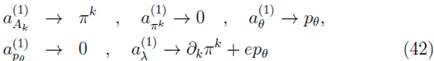
where

On these relations and Eq. (58), we immediately identify the generalized brackets as follow:

which are equivalents with (29) and (30).

Remarks and conclusions

In this paper we have analyzed the canonical structure of the gauge invariance Proca's electrodynamics. We have recover the gauge invariance adding a mass term with the help of an auxiliary field which has an appropriated gauge transformation. We constructed a consistent Hamiltonian formulation for the theory that includes the constraints and their algebra. The Hamiltonian that generates the evolution of the system and considers the full gauge freedom is determined. We studied the problem of gauge fixing for the theory, determining the appropriated gauge condition which result of the motion equations.

The fundamental Dirac brackets for the dynamical variables have been constructed and are compatible with the constraints.

In this paper we have studied Proca electrodynamics gauge invariance with the symplectic quantization method. We have shown that the symplectic approach is more intuitive in the sense that the constraints are related to the generalized canonical momenta and the Lagrange multipliers to the symplectic variables in the enlarged symplectic structure of the constrained manifold. For the Proca electrodynamics we have shown that the number of the constraints is fewer and the structure of these constraints is very simple because we do not need to distinguish first or second class constraints, primary or secondary constraints, etc. We have easily obtained the Dirac brackets by reading directly from the inverse matrix of the symplectic two form matrix. Finally, we can observe that the potential symplectic obtained at the final stage of iterations is exactly the Hamiltonian which is obtained through several steps with the usual Dirac formulation of the constrained systems.

Aknowledgements

BMP thanks CNPq for partial support. GERZ thanks VIPRI-UDENAR for full support.

A. Faddeev Jackiw formalism

We start by reviewing very briefly the Faddeev-Jackiw (FJ) quantization method ^[12,13] in field theories A general first order Lagrangian in time derivative is described by the symplectic variables ξ ^Α is given by

where ξ ¹ = ξ ¹ (x) = ξ ¹ (x, t) are the field variables. Based on the canonical one-form α _A (ξ) the symplectic matrix f _AB (x,y) is defined by

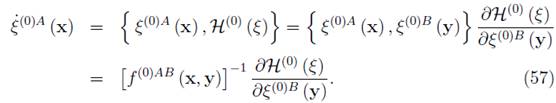
which is called the symplectic two-form. Generally, the geometric structure of the theory is fully described by the canonical generalized canonical momenta (ξ), and the symplectic matrix gives the geometric structure of the phase space. Using variational principle, we obtain the dynamical equations of motion:

Theories are classified as unconstrained and constrained depending on whether has an inverse or not, respectively. In the unconstrained case, when has an inverse, we can obtain the equations of motion such as

In this case, we can obtain the generalized symplectic brackets as

Compared (55) with (57) we have the relations between the symplectic two-form matrix and the generalized symplectic bracket

which correspond to the Dirac brackets ^[18].

When the symplectic matrix is singular leads us to constraints ^[14-16], which can be expressed as

where are the zero-modes associated to the matrix and α denotes the the number of constraints. The quantities Ω(α) are the constraints in the FJ symplectic formalism, and are introduced in the Lagrangian by using Lagrange multipliers:

In this point one can run the symplectic algorithm once again. Enlarging the configuration space by considering the set of variables ξΑ(1) = (ξ, λ(α)), by redefining the λ(α) variables, relating to we can set

therefore, the first iterated lagrangian is written as

where

In terms of the new set of dynamical variables ξA(1) one can now introduce a new symplectic matrix as,

If the matrix is regular, then we have succeeded in eliminating the constraints. If not, one should repeat the procedure above as many times as necessary. If we get the nonsingular f _AB after a finite number of iterations, we stop the iterations and obtain the generalized symplectic brackets from the inverse of f _AB, the brackets are exactly those the Dirac brackets. On the other hand, in some cases the iterations are repeated infinitely. In such a case, the zero mode plays an important role, generating a gauge symmetry. Then, we need some gauge fixing conditions Φ_σ with σ = 1, 2,... number of gauge conditions. Now, the basic spirit of the method is maintained exactly the same because the gauge fixing conditions are nothing but a kind of constraints. We may write the gauge fixed Lagrangian as follows:

where the subscript (k) denotes the iterations numbers the generate the modified symplectic matrix and the potential symplectic at the (k) iteration

The relation (64) is most general form of the first order Lagrangian. Note that the constraints and the gauge fixing conditions are considered as the generalized canonical momenta, while the Lagrangian multipliers are as their conjugated variables in the symplectic formalism. After following the procedure as above, we obtain the generalized symplectic brackets, which are the bridge to the quantum commutators.