Published
MASSLESS SCHWINGER MODEL IN THE NULL PLANE GAUGE
MODELO DE SCHWINGER SIN MASA EN EL GAUGE DE PLANO NULO
Keywords:
Null-plane coordinates, Massless Schwinger model, Constraint analysis, Null-plane gauge, Dirac brackets. (en)Coordenadas de plano nulo, Modelo de Schwinger sin masa, Análisis de vínculos, Gauge de plano nulo, Paréntesis de Dirac. (es)
The canonical commutation relations between the field and its canonical conjugate momenta can not be imposed on the null plane. It differs significantly from the instant form because a relativistic theory on null-plane describe a dynamical systems with constraints. We are going to study massless Schwinger Model on the null-plane coordinates using the null-plane gauge. The Dirac's procedure for constrained systems is used to perform a detailed analysis of the canonic structure of the theory. If we imposed appropriated boundary conditions on the fields and choose the null-plane gauge, we determined the generalized Dirac brackets of the independent dynamical variables which via the correspondence principle give the (anti)- commutators for posterior quantization.
Las relaciones de conmutación entre los operadores de campo y sus momentos canónicos no se pueden imponer directamente en las coordenadas de plano nulo. Este procedimiento difiere significativamente de su contraparte en las coordenadas en el instante forma, ya que una teoría relativista en las coordenadas de plano nulo describe un sistema dinámico con vínculos. Estudiaremos el modelo de Schwinger sin masa en las coordenadas de plano nulo y utilizaremos el método de Dirac para realizar un análisis detallado de la estructura canónica de la teoría. Si se consideran apropiadas condiciones de frontera sobre los campos y se impone la condición de gauge de plano nulo, se deducen los paréntesis de Dirac entre las variables dinámicas independientes las cuales, via principio de correspondencia, darán origen a los (anti) conmutadores para su posterior cuantización.
MASSLESS SCHWINGER MODEL IN THE NULL PLANE GAUGE
MODELO DE SCHWINGER SIN MASA EN EL GAUGE DE PLANO NULO
Germán E. Ramos-Zambrano1, Bruito M. Pimentel2, Juan B. Florez1
1Departamento de Física, Universidad de Nariño. Calle 18 Cra 50, San Juan de Pasto, Nariño, Colombia.
2Instituto de Física Téorica - Sao Paulo State University Caixa Postal 70532-2, 01156-970, São Paulo, SP, Brazil.
Contacto: Germán E. Ramos–Zambrano: gramos@udenar.edu.co
(Recibido: Mayo/2014. Aceptado: Junio/2014.)
Cómo citar: Ramos–Zambrano, G., Pimentel, B., & Florez, J., Momento. 48, 47 (2014)
Abstract
The canonical commutation relations between the field and its canonical conjugate momenta can not be imposed on the null plane. It differs significantly from the instant form because a relativistic theory on null–plane describe a dynamical systems with constraints. We are going to study massless Schwinger Model on the null-plane coordinates using the null–plane gauge. The Dirac's procedure for constrained systems is used to perform a detailed analysis of the canonic structure of the theory. If we imposed appropriated boundary conditions on the fields and choose the null-plane gauge, we determined the generalized Dirac brackets of the independent dynamical variables which via the correspondence principle give the (anti)– commutators for posterior quantization.
Keywords: Null–plane coordinates, Massless Schwinger model, Constraint analysis, Null–plane gauge, Dirac brackets
Resumen
Las relaciones de conmutación entre los operadores de campo y sus momentos canónicos no se pueden imponer directamente en las coordenadas de plano nulo. Este procedimiento difiere significativamente de su contraparte en las coordenadas en el instante forma, ya que una teoría relativista en las coordenadas de plano nulo describe un sistema dinámico con vínculos. Estudiaremos el modelo de Schwinger sin masa en las coordenadas de plano nulo y utilizaremos el método de Dirac para realizar un análisis detallado de la estructura canónica de la teoría. Si se consideran apropiadas condiciones de frontera sobre los campos y se impone la condición de gauge de plano nulo, se deducen los paréntesis de Dirac entre las variables dinámicas independientes las cuales, via principio de correspondencia, darán origen a los (anti) conmutadores para su posterior cuantización.
Palabras clave: Coordenadas de plano nulo, Modelo de Schwinger sin masa, Análisis de vínculos, Gauge de plano nulo, Paréntesis de Dirac.
Introduction
In 1949 Dirac pointed out that in a relativistic quantum theory the choice of the time variable is not unique [1] and he proposed three different forms of relativistic dynamics depending on the types of surfaces where independent modes were initiated. The first form, named instant form, when a space–like surface is chosen. It has been used most frequently so far and is usually called equal–time quantization. The second form, point form, is to take a branch of hyperbolic surface xμxμ=κ2,x0>0 and the last form, front form, is a surface of a single light wave. It is commonly referred to as null–plane formalism. This latter took almost 20 years before Dirac's idea of front form of dynamics was applied by physicist. At equal–time, any two different points are space–like separated and, therefore fields defined at these points are naturally independent quantities. For a null-plane surface the situation is different because the micro–causality principle leads to locality requirement in which only the transversal components and the appearance of any non–locality in the longitudinal coordinate in the theory would not be unexpected [2]. The null-plane coordinates are not related by a Lorentz transformation to the coordinates usually employed in the instant form and as such the descriptions of the same physical content in a dynamical theory on the null plane may come out be different from that given in the conventional treatment [3].
An important advantage pointed out by Dirac is that seven of the ten Poincaré generators are kinematical on the null–plane while in the conventional theory constructed on the instant form only six have this property. Other notable feature of a relativistic theory on the null–plane is that it gives rises to a singular Lagrangian, i.e., a constrained dynamical system [4, 5]. It leads in general to a reduction in the number of independent field operators in the corresponding phase space. It is illustrated in the present work by means of the analysis of the Schwinger model [6] .
Srivastava [3] studied the null–plane quantization of the bosonized version of the Schwinger model in the continuum formalism and he showed that the quantization of the massless Schwinger model leads in a straightforward way to the θ–vacua structure which is well–known to emerge [7] in the instant form analysis of the theory. He constructed a self–consistent Hamiltonian formulation, first separating the scalar field into the dynamical condensate and quantum fluctuations fields and obtained the correct mass for the Schwinger particle and reproduced correctly known features of the spectrum. Eller and Pauli [8] applied the method of discretized light–cone quantization to quantum electrodynamics in one space dimension and the spectrum of invariant masses and eigenfunctions of the light–cone hamiltonian was derived. Eller, Pauli and Brodsky [8] considered the case of massive and massless electrons, obtaining the correct mass for the Schwinger particle and reproducing correctly many known features of the spectrum. But, McCartor [9] showed that the last results is not a Schwinger model because they obtained a free massive scalar field once, rather that the standard result which shows an infinite number of degenerate copies.
The aim of the present work is to construct the Hamiltonian formulation of Massless Schwinger model on the null–plane description and to obtain a graded algebra among the fundamental dynamical variables of the theory. The constraint analysis shows the existence of hidden first–class constraints [10]. We are going to exhibit that when appropriate boundary conditions are imposed on the fields [11–13], this hidden first–class constraints are eliminated [14]. The boundary conditions ensure that the inverse of the second class matrix constraint is unique and well defined. We also show that if the projection of the fermionic fields is used, we observe the existence of only second class constraints in the fermionic sector and that the electron field is fully described by only one of its two components.
The work is organized as follow. We will analyze the constraint structure of the theory, next we classify the constraints and we impose the corresponding gauge fixing conditions. Also, we are going to study the dynamics of the fields using the extended Hamiltonian. Finally, we invert the constraints by imposing appropriate boundary conditions and the Dirac brackets (DB) of the theory are calculated. In the last section, we summarize the results obtained.
Structure of Constraints
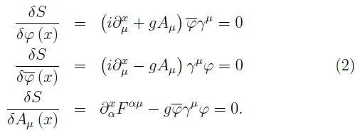
The Lagrangian density of Massless Schwinger model is defined by the following Lagrangian density1:

where the corresponding field equations are
The canonical theory on the null–plane is constructed defining the conjugate momenta to the fields ( φ, φ-. Aμ) as:
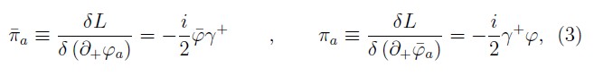
and
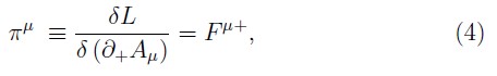
where, we have used left derivatives to define the field equations (2) and the canonical momenta associated to the fermions (3) 2. These equations show relations between coordinates and momenta, thus, from (3) and (4) we obtain a set of fermionic primary constraints
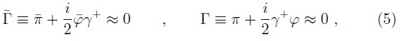
and the following bosonic primary constraint
![]()
Therefore, the Lagrangian density (1) describe a constrained system and we are going to use the Dirac's procedure [4, 5] to construct the graded algebra between the dynamical variables of the model to get a posteriori quantization via the correspondence principle. The canonical Hamiltonian density of the theory is defined by [15]:

consequently, the canonical Hamiltonian is: HC ≡ ∫dy ‾ HC. Following the Dirac's procedure [4, 5], we can construct the primary Hamiltonian HP adding to the canonical Hamiltonian the primary constraints with their respective Lagrange multipliers
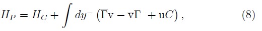
where v and v‾ are the respective multipliers associated to the fermionic constraints and u are the multipliers related to the electromagnetic constraints.
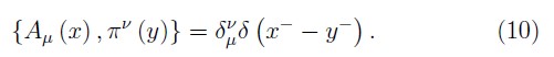
The fundamental Poisson Brackets (PB) among the the fermionic dynamical variables are defined by,

and, for the bosonic variables we have
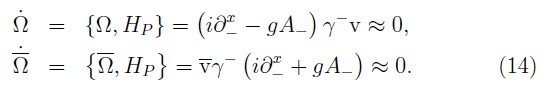
In order to the primary constraints are conserved under time evolution, we must calculate the PBs of them with the primary Hamiltonian HP . Thus, such requirement on the fermionic constraints (5) yields the following set of secondary constraints
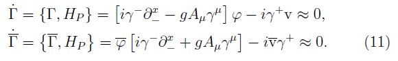
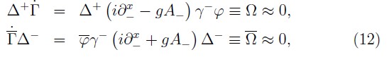
The relations given by (11) are conditions on the fermionic Lagrange multipliers, however, the singular nature of the γ+ matrix imply that not all components of v and v‾ can be determined. Thus, using the projector operators:3 Δ- and Δ+, a set of secondary constraints can be deduce:
and, some conditions for the components of the Lagrange multipliers

Now, the consistence condition on the secondary fermionic constraints (12) determines additional relations for all other components of the fermionic multipliers
Therefore, the equations (13) and (14) determine completely the fermionic multipliers and, we conclude that there are not more constraints associated with the fermionic sector.
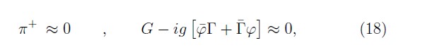
Alike, the consistence condition of the bosonic primary constraints (6) produces the following secondary constraint
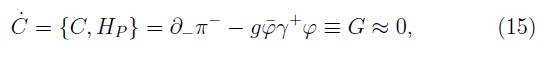
what is the Gauss's law, and its consistence condition shows that
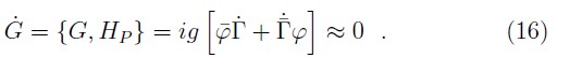
This implies that G is automatically conserved in time, then, no more constraints in the theory are generated.
Constraint classification
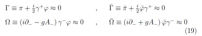
The constraint π+ has vanishing PB with all the other constraints, therefore, it is a first class constraint [4, 5]. The remaining set, Φa={Γ,Γ_,Ω,Ω_ is apparently a second class set, however, it is possible to show that their constraint matrix is singular and its zero mode eigenvector provides a linear combination of constraints which is a first class constraint. Alternately, we must observe that as the fermionic case, the electromagnetic sector must maintain its free constraint structure due that the interaction term is not allowed to change the first class structure of the free theory into second class ones, because the Dirac brackets would not be defined any longer in the limit of zero coupling constant. Thus, such combination, which is independent of π+ and it is a first class constraint, is:
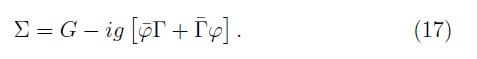
Then, we have the following subset of bosonic first-class constraints
and the subset of fermionic second-class constraints
with the following PB among them
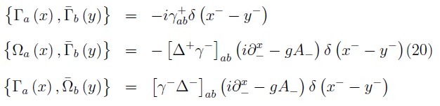
The null-plane constraint structure of the fermionic sector is the same that in the free case such as it was noted in [3, 16]. This result is not qualitatively different of that obtained when it is analyzed in the plane x0 = cte or instant form [17, 18] where the fermionic constraints are also of second class.
If we use the projection of the fermionic field, we observe from the fermionic second class constraints (12) that

Thus, the fermionic field is fully described by only one of two components. In [19] the analysis is performed without the projection of the secondary fermionic constraints, showing the existence of first-class constraint in the fermionic sector. We have shown that using the null-plane γ-algebra such first class set is really second class. As we will show in the next sections, the first class nature in the fermionic sector is related to the hidden subset of first-class constraints which generate improper gauge transformations [15] associated with the insufficiency of the initial value data and it implies that the matrix of the second-class constraints does not have a unique inverse. The hidden first-class constraints can be eliminated simply by fixing the necessary boundary conditions [11–13].
Now, the Dirac procedure said that we need of gauge conditions as there are first class constraints. Thus, we select as gauge conditions for the bosonic first class constraints (18) the following relations
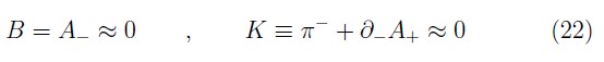
which are standard in the pure gauge theory (the so–called null–plane gauge) [20].
Equations of motion
At this point we need to check that we have the correct (Euler–Lagrange) equation of motions. First, one calculates the time derivative of the fields, where now the Hamiltonian that generates translations in the time is the extended Hamiltonian which is obtained adding to the total Hamiltonian HP all the first–class constraints of the theory
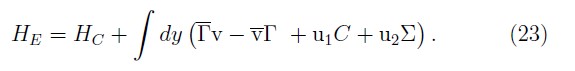
Thus, we get that the time evolution of the fermionic dynamical variables under HE are given by
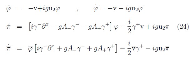
and for the electromagnetic field we have:
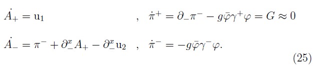
Using (24), for the fermionic fields it is easy to obtain that:
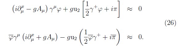
Alike, for the electromagnetic field it is possible to show:

Then, the equation of motions (26) and (27) are consistent with its counterpart Lagrangian form, (2), when we choose u2=0.
Dirac brackets
With the gauge fixing conditions (22), the first–class constraints are second–class. We procedure with the iterative method for the calculate of the Dirac brackets [17, 18]. For it, we first consider the following set of constraints
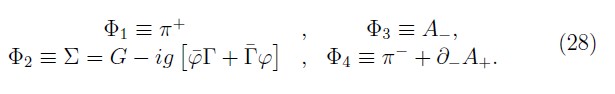
Thus, we define the first matrix constraints
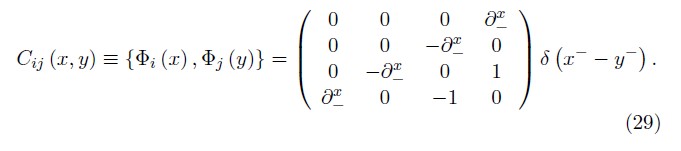
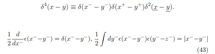
In order to solve the inverse of the constraint matrix, we require a suitable inverse of longitudinal derivative ![]() . In general
. In general
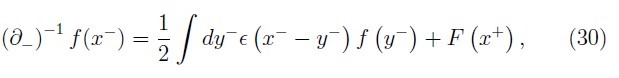
where ε(χ) = 1,0, —1 for χ ›, =,‹ 0, respectively and F (x+) is a x— independent function. The presence of F is associated with the insuficiency of the initial value data. This ambiguity implies that constraint matrix (29) does not have a unique inverse. Dirac has proved that the matrix formed by a complete set of second class constraints must have an unique inverse, thus, the set of second class constraints in (28) is not purely second–class. The matrix inverse of (29) is not unique because among the second class constraints there are a hidden subset first class constraints [10]. Steinhardt [14] shown that this hidden subset of first class constraints is associated with improper gauge transformations [10], which change the physical state of the system mapping one solution of the equations of motion onto a physically different one. Therefore, it is not possible to eliminate the improper gauge transformations by means of gauge conditions since such procedure would exclude configurations physically allowed to the system. This hidden constraints can be eliminated by fixing appropriated boundary conditions on the fields in order to the total Hamiltonian be a true generator of time evolution of the physical system.
Then, the explicit evaluation of the inverse of the matrix of second–class constraints involves the determination of an arbitrary function of (x+). This function can be evaluated by considering appropriate boundary conditions on the variations in the canonical
coordinates generated by the constraints. Then, if we impose the
boundary conditions on the fields (φ, ![]() Aμ) given by Neville and Rohrlich [2] [16], the inverse of the operator
Aμ) given by Neville and Rohrlich [2] [16], the inverse of the operator ![]() is defined on all integrable functions f)x–) which are less singular than
is defined on all integrable functions f)x–) which are less singular than![]() and vanish faster than
and vanish faster than ![]() for large x– by
for large x– by
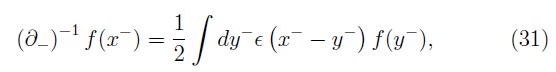
with this we get a unique inverse which is given as
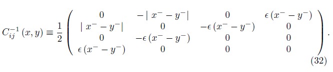
Using the inverse defined by equation (32), the first set of Dirac brackets for two dynamical variables Aa (x) and Bb (y) are calculate by,
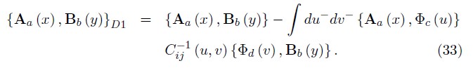
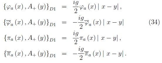
Thus, from (33) it is possible determine that the no null Dirac brackets D1 associated to the bosonic constraints are:
Now, we consider the subset of the remaining second class constraints that under the Dirac brackets D1 are given as:
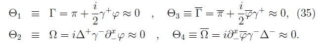
Next, the constraint matrix Dij (x, y) ≡ { Θi (x), Θj (y)} D1 of this set has the following components:
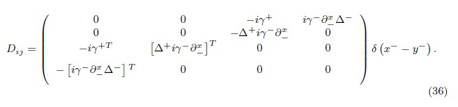
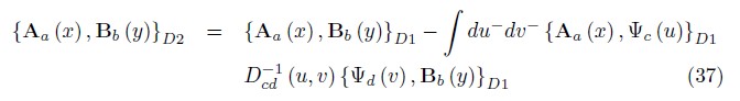
Using appropriate boundary conditions on the fields, we compute the inverse Dcd–1 (x,y) and thus we define the second set of DB,
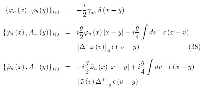
Then, we obtain the final Dirac brackets among the fundamental dynamical variables of the theory
Remarks and conclusions
We have performed the constraint analysis of the Massless Schwinger model on the null-plane and several characteristics or features are in contrast with the customary space–like hyper–surface formulation.
We have shown that the Massless Schwinger model has a first class constraint, the Gauss's law, which result of a linear combination of electromagnetic and primary fermionic constraints which is given by the zero mode eigenvector of the constraint matrix.
The careful analysis the constraints structure of the fermionic sector shows that it has only second class constraints. However, there exists a hidden subset of first class constraints [14] which generate improper gauge transformations [10]. Such first class subset are associated with the ambiguity in the definition of the inverse of the operator ![]() and with the deficiency of boundary conditions to solve the Cauchy data problem. Such ambiguities are eliminated by fixing the necessary boundary conditions on the fields.
and with the deficiency of boundary conditions to solve the Cauchy data problem. Such ambiguities are eliminated by fixing the necessary boundary conditions on the fields.
After select the null–plane gauge conditions to transform the first class constraints in second class one, we imposed appropriated boundary conditions on the fields to fix a hidden subset of first class constraints which allows to get an unique inverse of the second class constraints matrix. Following the Dirac's procedure, we obtain graded algebra (38) for the canonical variables.
Aknowledgements
BMP thanks CNPq and FAPESP (grant 02/00222-9) for partial support. GERZ thanks CNPq (grant 142695/2005-0) for full support.
A Appendix
A.1 Notation
We present here our notation with a few simple properties of the corresponding γ matrices.
The null plane time x+ and longitudinal coordinate x– are defined, respectively, as
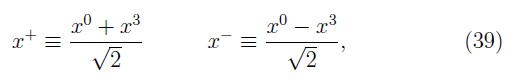
with the transverse coordinates ![]() ≡ (x1, x2) kept unchanged. Hence, in the space of four–vectors x = )x+, x11 x2, x–) , the metric is
≡ (x1, x2) kept unchanged. Hence, in the space of four–vectors x = )x+, x11 x2, x–) , the metric is
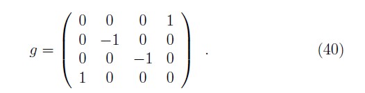
Explicitly,
![]()
where the derivatives with respect to x+ and x– are defined as
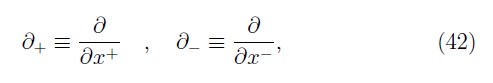
with ![]() =
=![]() . Here, we have used the following relations
. Here, we have used the following relations
The same orthogonal transformation is applied to Dirac matrices, which still obey
![]()
but with the new metric, this makes γ+ and γ–singular.
Since

we define the Hermitian matrices
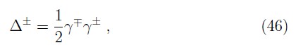
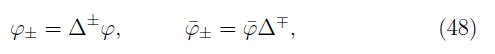
which are projection operators,
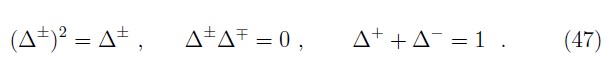
Their action on Dirac spinors yields
A.2 Grassmann Algebras
A Grassmann algebra contains bosonic (self–commuting) and fermionic (self–anticommuting) variables [21, 22]:
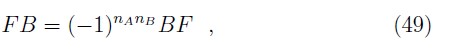
where n + 0 for a bosonic, and n + 1 for a fermionic variable. Note that the product of two fermionic variables is a bosonic one, and the product of a fermionic and bosonic variables is a fermionic one
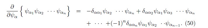
The left derivative of a ![]() fermionic variable is defined as
fermionic variable is defined as
The Poisson Bracket can be defined as similar to ordinary mechanics [23, 24]. The phase space is spanned by qi, pi which are bosons and ![]() and πα, fermions. Denote by B(F) a bosonic (Fermionic) element of the Grassmann algebra, then
and πα, fermions. Denote by B(F) a bosonic (Fermionic) element of the Grassmann algebra, then
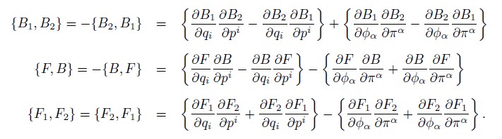
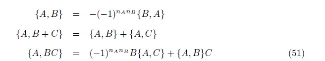
It follows from its definition that the Poisson bracket has the following properties
References
[1] P. Dirac, Rev. Mod. Phys. 21, 392 (1949).
[2] P. P. Srivastava, hep–th/9312064 (1993), CBPF–NF–075–93.
[3] P. P. Srivastava, hep–th/9610149 (1996), CBPF–NF–063–96, IF–UERJ–034–96.
[4] P. Dirac, Lectures on Quantum Mechanics, Belfer Graduate School of Science New York, NY: Monograph series (Belfer Graduate School of Science, Yeshiva University, 19640).
[5] A. Hanson, T. Regge, and C. Teitelboim, Constrained Hamiltonian systems: ciclo di lezioni tenute dal 29 aprile al 7 maggio 1974 , Contributi del Centro linceo interdisciplinare di scienze matematiche e loro applicazioni (Accademia Nazionale dei Lincei, 1976).
[6] J. Schwinger, Phys. Rev. 128, 2425 (1962).
[7] J. Lowenstein and J. Swieca, Ann. Phys. 68, 172 (1971).
[8] T. Eller, H.-C. Pauli, and S. Brodsky, Phys. Rev. D 35, 1493 (1987).
[9] G. McCartor, Z. Phys. C 41, 271 (1988).
[10] R. Benguria, P. Cordero, and C. Teitelboim, Nucl. Phys. B 122, 61 (1977).
[11] F. Rohrlich, Acta Phys.Austriaca Suppl. 8, 277 (1971).
[12] R. Neville and F. Rohrlich, Phys. Rev. D 3, 1692 (1971).
[13] R. Neville and F. Rohrlich, Nuovo Cimento A 1, 625 (1971).
[14] P. J. Steinhardt, Ann. Phys. 128, 425 (1980).
[15] P. Pyatov, A. Razumov, and G. Rybkin, (1988), IFVE-88-212.
[16] A. Das and S. Perez, Phys. Rev. D 70, 065006 (2004).
[17] K. Sundermeyer, Constrained Dynamics: with Applications to Yang-Mills Theory, General Relativity, Classical Spin, Dual String Model , Lecture Notes in Physics (Springer Berlin Heidelberg, 1982).
[18] A. Shirzad and P. Moyassari, hep–th/0112194 (2001), IUT–PHYS–01–11.
[19] D. Mustaki, Phys. Rev. D 42, 1184 (1990).
[20] E. Tomboulis, Phys. Rev. D 8, 2736 (1973).
[21] F. Berezin, The method of second quantization, Pure and applied physics (Academic Press, 1966).
[22] A. Kirillov, F. Berezin, J. Niederle, and R. Kotecký, Introduction to Superanalysis, Mathematical Physics and Applied Mathematics (Springer Netherlands, 2010).
[23] R. Casalbuoni, Nuovo Cimento A 33, 115 (1976).
[24] R. Casalbuoni, Nuovo Cimento A 33, 389 (1976).
1For notation see Appendix A.1
How to Cite
APA
ACM
ACS
ABNT
Chicago
Harvard
IEEE
MLA
Turabian
Vancouver
Download Citation
Article abstract page views
Downloads
License
Those authors who have publications with this journal, accept the following terms:
a. The authors will retain their copyright and will guarantee the publication of the first publication of their work, which will be subject to the Attribution-SinDerivar 4.0 International Creative Commons Attribution License that permits redistribution, commercial or non-commercial, As long as the Work circulates intact and unchanged, where it indicates its author and its first publication in this magazine.
b. Authors are encouraged to disseminate their work through the Internet (eg in institutional telematic files or on their website) before and during the sending process, which can produce interesting exchanges and increase appointments of the published work.