System Solver: an open source tool for mathematically modelling dynamical systems

System-Solver: una herramienta de código abierto para la modelación de sistemas dinámicos

The following paper presents a freeware modelling tool simulating dynamic systems that can be represented by either an ordinary differential equation (ODE) or a set of differential equations of different orders. The main idea leading to this software development is related to the fact that many physical, biological, ecological, economical, chemical, social and engineering problems can be expressed in this way. Furthermore, the solution to these problems requires some expertise in numerical methods and programming. Such knowledge is uncommon in some of the experts in such scientific domains. A tool to fill in this knowledge gap, increase productivity within modelling-related research and support the teaching of mathematical modelling topics is thus needed. This paper introduces System Solver, a computer application that facilitates the formulation of initial value problems for ODE systems, numerically solves these problems and provides a user with not only the solution but also debugged Visual Basic source code for the application. The obtained code can be easily shared among researchers, which facilitates the replication of numerical experiments even across different operating systems. This software's introduction is accompanied by examples from different domains, including one example from stochastic modelling.

En este artículo se presenta una herramienta de código abierto para la simulación de sistemas dinámicos, representados a través de ecuaciones diferenciales de distinto orden o de sistemas de ecuaciones diferenciales ordinarias (EDO). La idea principal que incentivó el desarrollo de esta herramienta consiste en que muchos procesos físicos, biológicos, ecológicos, económicos, químicos y sociales, y un sinnúmero de problemas ingenieriles, pueden ser expresados de esta forma. Adicionalmente, la solución de ese tipo de problemas exige experticia en métodos numéricos y programación. Este tipo de experticia no es muy común para los expertos de las áreas mencionadas; por ello, se requiere de una herramienta que permita sortear esta falta de experticia e incrementar la productividad en trabajos relacionados con tópicos de modelación. System-Solver es una aplicación que facilita la formulación de problemas de valor inicial en EDO y su solución numérica, y mediante un programa en Visual Basic la automatiza. El programa obtenido se puede compartir fácilmente con otros investigadores, facilitando la reproducción del ejercicio de modelación incluso en diferentes sistemas operativos. La presentación del software está acompañada con ejercicios de diversas áreas temáticas, incluyendo un ejemplo de modelación estocástica.

• HTML (es)
• HTML (en)

System-Solver: una herramienta de código abierto para la modelación de sistemas dinámicos System Solver: an open source tool for mathematically modelling dynamical systems

Efraín Domínguez¹, Felipe Ardila² y Santiago Bustamante³

¹ Ingeniero Hidrólogo. M.Sc., en ecología hidrometeorologia. Ph.D., en ciencias técnicas. Universidad Javeriana, Bogotá, Colombia. e.dominguez@javeriana.edu.co

² Ingeniero de Ssitemas, Universidad Distrital. Estudiante de M.Sc., en Hidrosistemas, Universidad Javeriana, Bogotá, Colombia. Instituto Geofísico. felipeardilac@gmail.com.

³ Pregrado, Universidad Javeriana, Bogotá, Colombia. santiagobus@gmail.com

---

RESUMEN

Palabras claves: ODE Solver, diferenciación por computadoras, modelación, sistema dinámicos.

---

ABSTRACT

Keywords: ODE solver, computational differentiation, modelling, dynamical system.

---

Recibido: junio 23 de 2009
Aceptado: noviembre 15 de 2010

Introducción

 Muchos problemas del mundo real pueden ser estudiados utilizando modelación matemática. El operador diferencial es una herramienta matemática ampliamente utilizada para describir procesos físicos, biológicos, ecológicos, etcétera. Usualmente el problema en estudio se describe a través de una EDO de orden r o a través de un sistema de EDO. Y con frecuencia la solución de esa ecuación, o sistema de ecuaciones, se establece con la aplicación de métodos numéricos. Los interesados en solucionar numéricamente un modelo matemático deben estar familiarizados con lenguajes de programación y algoritmos numéricos. Sin esta experiencia el proceso de investigación del modelo matemático se retrasa hasta que haya disponibilidad de un especialista en las áreas mencionadas.

La integración automática de sistemas de EDO siempre ha sido un tema de interés para la comunidad científica. El desarrollo de esta temática comenzó en 1970 (Moore, 1979). Tolsma y Barton (1998) sugieren cinco aproximaciones para la derivación computacional: 1) codificación manual, 2) aproximación por diferencias finitas, 3) derivación simbólica, 4) aplicación de la notación polaca inversa (RPN, por su sigla en inglés) (Bardsley y Prasad, 1997), 5) diferenciación automática. Iri (1991) postuló los prerrequisitos de un buen método de integración: debe ser rápido, libre de error de truncamiento y preferiblemente aplicado en forma automática. Adicionalmente, se requiere añadir otro prerrequisito: el método a utilizar debe permitir su generalización a sistemas de cualquier complejidad. De los métodos enunciados, el quinto y el sexto cumplen con casi todos los requerimientos planteados. El error de truncamiento se mantiene presente en el segundo método. El quinto método requiere alta intervención del usuario, quien debe programar un procedimiento inicial para iniciar la integración de un sistema de EDO concreto. Adicionalmente, la diferenciación automática puede requerir algún esfuerzo de adaptación de código para resolver problemas planteados en forma discreta (tabulada). Los métodos mencionados se aplican en la solución de problemas de modelación para variadas áreas científicas, y usualmente todas estas técnicas son estudiadas en cursos estandarizados de modelamiento matemático. En el mercado hay una cantidad considerable de programas especializados en la solución de sistemas de EDO. La mayoría de éstos son de licencia privativa y se pueden acceder sólo comprándolos y generalmente no son transparentes para el usuario en el sentido de los algoritmos utilizados, ya que no proveen libre acceso al código fuente de los algoritmos preprogramados en ellos.

Este artículo ofrece los fundamentos teóricos, métodos, algoritmos, y la implementación de un programador automático de soluciones numéricas para sistemas de EDO. Dicho sistema de modelación implementa los métodos explícitos de Euler y Runge–Kutta y exporta la solución numérica para visualización en Scilab o Matlab. Tal aplicación representa la primera versión de un sistema de modelamiento que implementa la generación automática de programas que resuelven ecuaciones deferenciales para el estudio de sistemas complejos.  

System–Solver es una herramienta de distribución gratuita, recomendada para personas que quieren resolver EDO en forma numérica pero que no son programadores. Su aplicación es más fácil de usar que programas como Matlab porque no requiere conocimientos de programación, usa pocos comandos y está diseñada específicamente para resolver sistemas de EDO. System-Solver es un software pedagógico de alta calidad para la introducción al mundo de la modelación. La ventaja de usarlo en lugar de los bien conocidos Matlab, Scilab u Octave consiste en su diseño, orientado a la enseñanza. Este diseño permite desarrollar habilidades programadoras y de modelación matemática a la vez. Otra ventaja potencial reside en la posibilidad de escoger el lenguaje de programación que el usuario desea aprender y utilizar para compartir los programas de los sistemas modelados. Dicha habilidad será habilitada en la siguiente versión del paquete.  

System-Solver se creó en Java utilizando una librería especializada llamada Qt Jambi, una tecnología con soporte oficial para programadores que desean crear interfaces gráficas muy ricas aplicando código en lenguaje Java.

Comparado con herramientas de modelamiento conceptual como Stella, Powersim, Simile o Vensim, System-Solver explica en forma más clara los conceptos básicos en modelación. De hecho, un usuario puede ver las EDO que explican el sistema que se modela, y también tiene el control total del código numérico desarrollado para el sistema en estudio. El diseño de problemas n-dimensionales en modelamiento conceptual puede ser problemático a través de la representación visual del diagrama para el problema propuesto. La estructura de System–Solver fue diseñada para permitir la configuración amigable de sistemas n-dimensionales, de modo que se facilite la modelación de sistemas distribuidos.

Estructura de System-Solver

Se propone la siguiente notación:

El sistema (1) sugiere un algoritmo cíclico que aplique un método numérico (Euler o Runge-Kutta en nuestro caso) n-veces para encontrar el vector y (Боглаев, 1990). System-Solver implementa un esquema de diferencias finitas explícitas de Euler como el siguiente:

También es posible seleccionar un esquema explícito de Runge-Kutta de cuarto orden de la forma:

En ambas ecuaciones [(2) y (3)], n_i^j representa un error inducido por el truncamiento de las derivadas de alto orden en la serie de Taylor durante la deducción de las diferencias finitas para la EDO j. De hecho, n_i→0 si Δx→0. Los esquemas (1) y (2) son explícitos, y su desempeño depende fuertemente del tamaño del paso Δx. El índice i fija el nodo x que está siendo evaluado.

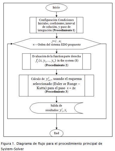
Para un programador experimentado es fácil reconocer un comportamiento genérico en las ecuaciones (1), (2) y (3) para la solución de un sistema de EDO. También se debe tener una rutina para evaluar y^j_i+1 (procedimiento 3 en la Figura 1), y la parte derecha de la ecuación (1) debe resolverse con un procedimiento externo (2 en la Figura 1). La configuración de condiciones iniciales, del intervalo de solución, los coeficientes de la EDO y el paso de integración (Δx deben ser especificados. Esto puede realizarse al comienzo de los cálculos (procedimiento 1 en la Figura 1). Para resolver la función de la parte derecha se implementó un procedimiento parcelador de ecuaciones que permite identificar las variables requeridas y los parámetros de la EDO. Estos parámetros también pueden ser función del tiempo o de las variables de estado del sistema (1).

En la Figura 2 se muestra la estructura básica de System-Solver. Esta estructura propone una interface para configurar la cantidad de ecuaciones en el sistema de EDO y campos para las expresiones que definen las funciones de la parte derecha de las EDO. Un método llamado "Solve" activa la traslación de la notación algebraica hacia la notación de registro polaco inverso (RPN). De la cadena de caracteres RPN se deducen y clasifican los parámetros, las variables independientes y variables de estado, que son insertados en una plantilla de código preparado previamente. La primera plantilla (RPEvaluator) evalúa las funciones de la parte derecha.

Una vez se rellena la plantilla RPEvaluator con el número correcto de variables y los parámetros requeridos por la EDO, se completa otra plantilla con el intervalo de discretización, vectores de condiciones iniciales y el número de pasos en el tiempo. EDOSystem es la implementación del diagrama de flujo presentado en la Figura 1. Este procedimiento es el subprograma principal que invoca una instancia de RPEvaluator, el cual retorna un vector solución para las funciones de la parte derecha requerido por los subprocedimientos Runge-Kutta o Euler y se crea una nueva evaluación de y^j_i+1 para cada nodo de tiempo x.

Como ejemplo, se examinan algunos sistemas dinámicos y se compara el código generado por System-Solver contra el código escrito a mano por un programador. Considérese un sistema predador-presa del siguiente tipo:

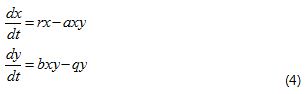
Donde r y q son los coeficientes de crecimiento, mientras que ay b son las tasas de beneficio por ataque del predador y la tasa de perjuicio de la presa, respectivamente.

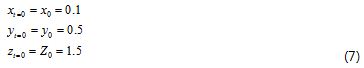
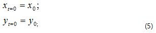
Dadas las siguientes condiciones iniciales,

Un modelador experimentado encontraría la solución numérica de (4) utilizando el método de Euler.

Siguiendo la estructura propuesta en la Figura 1, el procedimiento Sistema_ODE_Euler es equivalente al procedimiento 1 en la Figura 1; el procedimiento de la subderecha (…) equivale al procedimiento 2, y el subprograma Euler (…) evalúa x_t+1 y y_t+1 (procedimiento 3 en la Figura 1).

Para resolver el mismo problema en System-Solver se debe configurar el sistema EDO añadiendo cada ecuación usando la notación algebraica comúnmente aplicada en hojas de cálculo para definir fórmulas. El orden del sistema EDO está limitado sólo por las capacidades computacionales del ordenador. La Figura 2 describe la ventana principal de System-Solver. Esta aplicación ofrece una interface amigable incluso para investigadores con mínima experiencia en modelación, métodos numéricos y programación. La configuración de un modelo requiere no más de un par de minutos. El investigador debe invertir su tiempo encontrando las ecuaciones necesarias para su sistema, definiendo los valores de los parámetros en estas ecuaciones e interpretando resultados, en lugar de gastarlo definiendo, codificando y depurando el código de un algoritmo numérico.

Para el caso del modelo predador-presa (ecuación 4), System-Solver genera el código en Visual Basic, que se puede consultar en http://www.mathmodelling.org/home/system-solver-1.

El código Visual Basic generado por System-Solver puede ser copiado directamente en un módulo Visual Basic de Microsoft Excel para ser utilizado como un macro guardado directamente en un libro de Excel. El código generado también puede ser preparado para el compilador de Microsoft Visual Basic (versión Stand Alone). Una versión gratuita de este compilador se puede obtener desde el sitio web http://www.microsoft.com. Adicionalmente, el proyecto de código abierto "Mono" financiado por Novell incluye un compilador de Visual Basic, con entorno de desarrollo integrado, que puede ser ejecutado en diferentes sistemas operativos, incluyendo: Linux, Mac OS X, Sun Solaris, BSD - OpenBSD, FreeBSD, NetBSD y Microsoft Windows. (Más información sobre el proyecto "Mono", en: http://www.mono-project.com).

Si el código generado por System-Solver es preparado para la versión Stand Alone del compilador de Microsoft Visual Basic, se deberá editar el código para implementar procedimientos de pre y posprocesamiento. Independientemente de la plataforma para la cual fue generado el código, las herramientas Scilab y Matlab ofrecen una opción de posprocesamiento. System-Solver puede guardar los resultados del experimento numérico en formato ASCII y generar automáticamente el script que realizará la salida gráfica en los entornos de Scilab o Matlab.

Muchos problemas de modelación incluyen sistemas de tres o más EDO para describir los sistemas reales que se estudian. Estos sistemas multidimensionales requieren gráficas 3D para el posprocesamiento. En este caso System-Solver ofrece una opción para exportar resultados, la cual los prepara para ser procesados con Scilab o Matlab. La solución discreta se guarda en un archivo de texto y luego se importa en Scilab o Matlab con un script generado por System-Solver. Para examinar esta opción se resuelve el siguiente sistema predador-presa 3-dimensional (Sáez et al., 2007):

Con las siguientes condiciones iniciales:

y utilizando los siguientes parámetros: a=1.5, b=5.0, c=8.0,q=1.0, f=0.16, g=0.1, w=1.1 , l=2.0, m=0.16, Δt=0.1, t_min=0,t_max=500. Desarrollando esta configuración en System-Solver se obtiene el código Visual Basic presentado en la Figura 2.

La función "export" de System-Solver guarda los resultados y genera un script de Scilab en una ubicación seleccionada por el usuario. El script generado por System-Solver se presenta en la Figura 3.

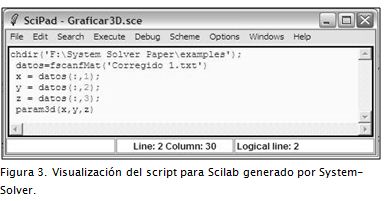
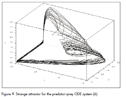
Cargando y ejecutando este script en el entorno de Scilab, se produce la gráfica presentada en la Figura 4.

Conclusiones

Los ejemplos presentados aquí muestran que el primer prototipo de System-Solver es capaz de manejar problemas EDO de diferente complejidad. Esta versión puede generar programas de soluciones numéricas eficientes y tiene herramientas para exportar los resultados de los experimentos numéricos a Scilab o Matlab, habilitando posprocesamiento 3D de los resultados. Esa aplicación ofrece una herramienta útil para el modelamiento de sistemas representados por conjuntos de EDO, acelerando la investigación relacionada a sistemas de EDO. System-Solver también puede acompañar los esfuerzos de enseñanza en curso de modelación matemática, programación y métodos numéricos. Usar System-Solver cierra el ciclo de definición del modelo matemático, desarrollo del algoritmo numérico y codificación del programa para la simulación de un sistema dinámico (Samarsky y Mikhailov, 1997).

La facilidad de System-Solver para aplicar el método de Euler, o el de Runge-Kutta de cuarto orden, permite la exploración de sus propiedades para el sistema de EDO investigado.

SystemSolver se desarrolla como herramienta multiplataforma. Se proyecta que las futuras versiones generen código para diversos compiladores como: C#, C++, Java, Object Oriented Pascal, Component Pascal y Fortran. En este momento el código generado se escribe para compiladores de Visual Basic (como el incluido en las aplicaciones de MS Office). Un compilador de Visual Basic está disponible en el proyecto "Mono", por ello el código Visual Basic generado por System-Solver también puede ser ejecutado en Linux y otros sistemas operativos. Una versión beta de System-Solver puede descargarse gratuitamente desde: http://www.mathmodelling.org/home/system-solver-1.

Se proyecta que distintos algoritmos numéricos de solución de sistemas EDO, incluidos algoritmos para ecuaciones rígidas, serán implementados en System-Solver en el futuro cercano. Algoritmos para la solución de ecuaciones diferenciales estocásticas están siendo asimilados. Las sugerencias con requerimientos de los usuarios de System-Solver también son bienvenidas.

Bibliografía

Bardsley, W.G., Prasad, N., Using ASCII text files in post-fix notation (reverse Polish) to define mathematical models and systems of differential equations for simulation and non-linear regression., Computers & Chemistry, 21(2), 1997, pp. 71-82.

Iri, M., History of automatic differentiation and rounding error estimation., Automatic differentiation of algorithms: Theory, implementation and application. SIAM, Philadelphia, PA., 1991.

Moore, R.E., Methods and applications of interval analysis., SIAM Publications, Philadelphia, 1979.

Saez, E., Stange, E., Szanto, I., Chaotic Dynamics and Coexistence in an Interaction Model Between Three Species., Universidad Técnica Federico Santa María - Departamento de Matemáticas, 2007, pp. 5.

Samarsky, A., Mikhailov, A., P., Matematicheskoie modelirovanie: Idei, metodi, primieri., Nauka, Moscow, 1997, 316 pp.

Tolsma, J.E., Barton, P.I., On computational differentiation., Computers & Chemical Engineering, 22(4-5), 1998, pp. 475-490.

Боглаев, Ю.П., Вычислительная математика и програми-рование, 1. Высшая школа, Москва, 1990, 544 pp.

System Solver: an open source tool for mathematically modelling dynamical systems

Efraín Domínguez¹, Felipe Ardila² y Santiago Bustamante³

¹ Hydrologist Engineer. M.Sc., in ecology Hydrometeorology. Ph.D., in technical sciences. Universidad Javeriana, Bogotá, Colombia.e.dominguez@javeriana.edu.co

² Systems Engineering, Universidad Distrital. M.Sc., student in Hydrosystems, Universidad Javeriana, Bogotá, Colombia. Geophysical Institute. felipeardilac@ gmail.com.

³Undergraduate, Universidad Javeriana, Bogotá, Colombia. santiagobus@gmail.com

---

ABSTRACT

The following paper presents a freeware modelling tool simulating dynamic systems that can be represented by either an ordinary differential equation (ODE) or a set of differential equations of different orders. The main idea leading to this software development is related to the fact that many physiccal, biological, ecological, economical, chemical, social and engineering problems can be expressed in this way. Furthermore, the solution to these problems requires some expertise in numerical methods and programming. Such knowledge is uncommon in some of the experts in such scientific domains. A tool to fill in this knowledge gap, increase productivity within modelling-related research and support the teaching of mathematical modelling topics is thus needed. This paper introduces System Solver, a computer application that facilitates the formulation of initial value problems for ODE systems, numerically solves these problems and provides a user with not only the solution but also debugged Visual Basic source code for the application. The obtained code can be easily shared among researchers, which facilitates the replication of numerical experiments even across different operating systems. This software´s introduction is accompanied by examples from different domains, including one example from stochastic modelling.

Keywords: ODE solver, computational differentiation, modelling, dynamical system.

---

Received: june 23th 2009

Accepted: november 15th 2010

Introduction

Several real world problems can be studied using mathematical modelling methods. The differential operator is a widely-used operator for describing physical, biological, ecological and other types of processes. These processes are usually described through either an ODE of a different order r or a set of ODEs. Resolving these equations or sets of equations is often done by using numerical methods. For researchers interested in numerical solutions to their mathematical models, one has to be familiar with both numerical and programming techniques; however, this requirement delays research unless a specialist in numerical methods becomes available).

Automatic integration of ODE systems has been of interest for a long time. In fact, computational differentiation development (Tolsma and Barton, 1998) has been happening since the 1970s (Moore, 1979). Tolsma and Barton (1998) suggested five approaches to the computation of derivatives: hand-coding, finite-difference approximation, symbolic differentiation, evaluation using Reverse Polish Notation(RPN) (Bardsley and Prasad, 1997) and automatic differentiation. Iri (1991) described some prerequisites for a good differentiation method; it should be fast, free of truncation error and preferably performed automatically. Perhaps, however, an additional prerequisite should be considered. The method must allow generalisation to systems of any complexity. The second and fifth methods almost fulfil all of the mentioned requirements. Truncation errors are still present in the second method, however, and the fifth method requires high user intervention for providing a starting subroutine for calculating a given ODE system. Automatic differentiation could require some adaptation for solving problem sets in a discrete (tabular) manner. All of the above-mentioned techniques are used for solving modelling problems in different science domains and all of them are usually studied within the standard programme of a mathematical modelling course. There is a significant amount of specialised software on the market for solving ODE systems; most of this software is not available free of charge, however, and not all of the algorithms used are known as clearly as the researchers wish. The available applications do not provide the source code for the ODE system being investigated.

This paper presents the theoretical foundations, methods, algorithms and implementation of an automatic programmer and numerical solver for ODE Systems. This modelling system uses both Euler and Runge-Kutta explicit methods and export numerical solutions for visualisation within Scilab or Matlab packages. This application represents the first version of a modelling system implementing automatic code generation for solving differential equations when studying complex systems.

System Solver is open source software. It is a good tool for people who like to solve ODE although they are not programmers. This application is easier to use than programmes like Matlab because it only uses a few commands and it is specifically designed to solve ODE. System Solver is high-quality pedagogical software for an introduction to the world of mathematical modelling. The advantage of using System Solver instead of known programmes such as MatLab, Scilab or Octave is the teaching-orientated design aimed at developping modelling and programming skills at the same time. Another potential advantage is the possibility of choosing the language programme that users want to learn for modelled systems share code; such ability will be implemented in the next version of the package.

System Solver was developed in Java script and uses a special library named "Qt Jambi." It is an officially-supported technology aimed at all programmers who want to write rich GUI clients using Java language.

Compared to conceptual modelling tools like Stella, Powersim, Simile or Vensim, System Solver shows better explanatory power for basic modelling concepts. System Solver users can see the ODE behind the system they are simulating and they also have total control over a numerical code being used for solving the ODE system being studied. The design of n-dimensional problems in conceptual modelling systems can be troublesome because of the visual representation of the problem diagram. System Solver structure has been designed to allow a friendly setup of n-dimensional systems and the assimilation of partial differential equations to model distributed systems.

System-Solver structure

Using the following notation:

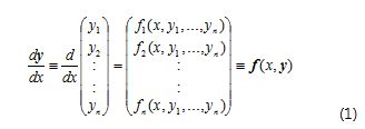
System (1) suggests a cyclical algorithm that applies a numerical method (Euler or Runge-Kutta in this case) ⁿ -times to find vector ^y (Боглаев, 1990). System Solver uses the Euler explicit finite differences scheme as follows:

It is also possible to select a fourth order Runge-Kutta explicit scheme in the form:

In both equations [(2) and (3)], n_i^j  represents an induced error due to the truncation of high order Taylor series derivatives during the deduction of finite differences for the ODE j . In fact,n_i→0 si Δx→0. Schemes (1) and (2) are both explicit and their performance depends heavily on the size of steps Δx. Index ⁱ fixes the ^x node that is being evaluated.

An experienced programmer will easily to recognise generic behaviour in equations (1), (2), and (3) for solving an ODE system. There must be a routine for evaluating y^j_i+1 (procedure 3 in Figure 1) and the right side of eq. (1) has to be solved using an external procedure (2 in Figure 1). The initial conditions, solution interval, ODE coefficients and integration step (Δx  ) must be setup. This can be done at the beginning of the calculations (procedure 1 in Figure 1). To solve the right side of functions, a parser procedure has been implemented leading to the identification of required variables and ODE parameters; ODE parameters can also be a function of time and/or the state variables of the system (1)

The basic System Solver structure is shown in Figure 2. This structure provides an interface for setting both the quantity of ODE in the studied system and also the fields for expressions defining right parts of the functions. A method called "Solve" activates the translation from algebraic notation to reverse Poland notation (RPN). The parameters, independent variables and state variables are classified from the RPN strings and used in previously-prepared code templates. The first template (RPEvaluator) evaluates the right parts of the expressions.

Once the RPEvaluator template is filled with the correct number of variables and the required ODE parameters, another template (EDOSystem) is completed with discretisation intervals, initial condition vectors and number of time steps. The EDOSystem is the implementation of the flow scheme presented in Figure 1. This procedure is the main procedure invoking a RPEvaluator instance that returns a solution vector for right parts of the equation required by the Runge- Kutta or Euler procedures and creates a new evaluation y^j_i+1  for every time node ^x .

Some dynamic systems are examined and their hand-code and System Solver solutions compared as an example. Consider a predator-prey system of the type:

Here, ^r and ^q are growth coefficients and ^a and ^b are the predator´s attack rate and its reproductive efficiency, respectively.

Given initial conditions,

An experienced modeller would find the numerical solution of (4) using the Euler methods.

Following the structure shown in Figure 1, the ODE_Euler system is equivalent to Procedure 1 in Figure 1, the sub right(.) is the equivalent of Procedure 2, and the sub Euler(.) evaluates x_t+1  and   y_t+1  y (procedure 3 in Figure 1).

The ODE system must be set up to solve the same problem within the System Solver application by adding each equation at once using the common notation used in spreadsheet applications to define mathematical expressions. The order of the ODE system is only restricted by the hardware specifications. Figure 2 describes the main System Solver window. This application is user-friendly, even for scientists having minimal knowledge of modelling, numerical methods, and programming. A model setup requires no more than a couple of minutes to complete. The researcher expends time in finding the required equations, defining the numerical values of parameters and interpreting results instead of designing, coding and debugging a numerical algorithm.

For the case of the predator-prey model (Equation 4), System Solver provides the Visual Basic code shown in http://www.mathmodelling.org/home/System Solver-1

The System Solver Visual Basic code can be pasted directly to a Microsoft Excel Visual Basic module. It can then be used as a Macro to obtain model results placed directly into a sheet in the current Workbook. The generated code can also be prepared for the MS Visual Basic stand alone compiler. This compiler can be downloaded from the Microsoft web site: http://www.microsoft.com. The open source "Mono" project sponsored by Novell has included a Visual Basic compiler in its integrated development environment. This compiler allows MS Visual Basic code to run in different operating systems, including Linux, Mac OS X, Sun Solaris, BSD - OpenBSD, FreeBSD, NetBSD and Microsoft Windows. More information about the "Mono" project can be obtained from: http://www.monoproject.com.

If the System Solver code is generated for a stand-alone Visual Basic compiler, it is necessary to edit the output code to permit post-processing. Independently of the platform for which the code is generated, the Scilab or Matlab packages offer one post-processing option. System Solver can save numerical results to an ASCII formatted text file and generate the required script to provide rapid graphic output in Scilab or Matlab environments.

Solving a third order ODE system and exporting the results to the Scilab and Matlab packages

Many modelling problems include three or more ODEs in the system to describe a phenomenon being studied. Such multidimensional systems require 3D graphic abilities during post-processing. In the System Solver case, such abilities are provided by the export option which prepares the results to be processed with the Scilab or Matlab packages. The discrete solution is exported to a text file and an import script that imports the resulting data to the selected package (Scilab or Matlab) is provided. A three-dimensional competition model given by the system can be solved to examine this ability (Saez et al., 2007):

with initial conditions:

using the following parameters: a=1.5, b=5.0, c=8.0,q=1.0, f=0.16, g=0.1, w=1.1 , l=2.0, m=0.16, Δt=0.1, t_min=0, and. Entering this setup into System Solver provides us with the Visual Basic code listed in Figure 2.

The Solver System "export" function saves the resulting data and a Scilab script within a user-selected location. The script is presented in Figure 3.

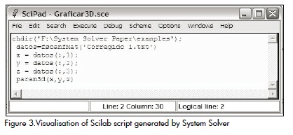
Loading and executing the Script in the Scilab environment produces the graphing shown in Figure 4.

Conclusions

The examples presented show that the System Solver prototype is able to handle ODE and PDE problems of differing complexities. This version can write efficient numerical code and provides tools for exporting the numerical results to Scilab and Matlab programmes enabling 3D graphical presentation of problem output. The application presented here offers a helpful tool for modelling systems represented by sets of ODEs. All of these abilities accelerate research when dealing with ODE systems and they also support teaching efforts in programming, mathematical modelling and numerical methods courses. Using System Solver closes the cycle of defining a mathematical model, building a numerical algorithm and coding a programmeto simulate a dynamic system (Samarsky and Mikhailov, 1997).

System Solver´s ability to switch between the Euler and fourth order Runge-Kutta methods allows exploring their properties for each ODE system investigated.

System Solver has been thought to act as a cross platform system. It is projected that future System Solver versions will provide source code for several compilers, such as C#, C++, Java, object-oriented Pascal, component Pascal and Fortran compilers. At the moment,output source code is written for Visual Basic compilers and Visual Basic for applications interpreters (like the one included in MS Office applications). A Visual Basic compiler is also available for the Mono project so the produced code can also be executed in Linux and other UNIX-like systems. A beta version of System Solver can be downloaded from the website: http://www.mathmodelling.org/home/System Solver-1

It is envisioned that several numerical algorithms for solving ODE systems, including algorithms for stiff (rigid) equations, will be provided by System Solver in the near future; algorithms for solving stochastic differential equations will also be implemented. Suggestions regarding user requirements from System Solver users are welcome.

References

Bardsley, W.G., Prasad, N., Using ASCII text files in post-fix notation (reverse Polish) to define mathematical models and systems of differential equations for simulation and non-linear regression., Computers & Chemistry, 21(2), 1997, pp. 71-82.

Iri, M., History of automatic differentiation and rounding error estimation., Automatic differentiation of algorithms: Theory, implementation and application. SIAM, Philadelphia, PA., 1991.

Moore, R.E., Methods and applications of interval analysis., SIAM Publications, Philadelphia, 1979.

Saez, E., Stange, E., Szanto, I., Chaotic Dynamics and Coexistence in an Interaction Model Between Three Species., Universidad Técnica Federico Santa María - Departamento de Matemáticas, 2007, pp. 5.

Samarsky, A., Mikhailov, A., P., Matematicheskoie modelirovanie: Idei, metodi, primieri., Nauka, Moscow, 1997, 316 pp.

Tolsma, J.E., Barton, P.I., On computational differentiation., Computers & Chemical Engineering, 22(4-5), 1998, pp. 475-490.

Боглаев, Ю.П., Вычислительная математика и програми-рование, 1. Высшая школа, Москва, 1990, 544 pp.